
Effects of Hydrologic Pulsing and Vegetation on Invertebrate Communities in Wetlands
Capital University, Columbus, OH 43209, USA
Land 2022, 11(9), 1554; https://doi.org/10.3390/land11091554
Submission received: 28 July 2022
/
Revised: 29 August 2022
/
Accepted: 8 September 2022
/
Published: 13 September 2022
(This article belongs to the Special Issue Wetland Construction and Restoration: Design and Performance)
Abstract
:Constructed, mitigation wetlands in the midwestern United States are frequently dominated by a Typha spp. monoculture and their hydrologies are often determined by adjustable control structures. Wetlands provide habitat for multiple macroinvertebrate species, which in turn provide food for other organisms inhabiting the wetlands, such as waterfowl. This study examined the impacts of plant diversity and manipulated hydrology on macroinvertebrate communities. Forty 1-m2 wetland mesocosms were either planted with a monoculture of Typha spp. or with a more diverse plant community of Schoenoplectus tabernaemontani, Juncus effusus, and Sparganium eurycarpum. They were also assigned to one of four hydrologic regimes: steady state, pulsing, deep spring/shallow fall, and shallow spring/deep summer. After one year, macroinvertebrates were sampled in the mesocosms. Mesocosms with deep spring hydrologies were found to have greater taxon diversity than those with other hydrologies, but Chironomidae biomass was the lowest under the deep spring hydrology. Culicidae and Chironomidae were found in higher numbers in mixed vegetation than in Typha spp. Taxon richness and Chironomid biomass were significantly higher in mixed vegetation mesocosms than in Typha spp. monocultures. Results suggest vegetation diversity and hydrological regimes impact macroinvertebrate communities, with potential implications for constructed wetland design and management.
1. Introduction
Wetland macroinvertebrates are a key component of wetland ecosystems. They contribute to nutrient processing and are important food for a variety of organisms—notably waterfowl [1,2]. Batzer and Wissinger [3] identify multiple studies that indicate the importance of aquatic invertebrates, particularly Chironomidae among the insects, as a food source for ducks.
The roles of plant communities and wetland hydrology in shaping macroinvertebrate populations in wetlands has significant implications for constructed wetland design and management. This study builds on the body of data collected thus far on the relationships between macroinvertebrate populations and the macrophyte communities and hydrology of wetlands.
Conventional wisdom claims, “Increasing habitat heterogeneity has direct and positive impacts on the aquatic biota. For example, food availability and habitat are provided for aquatic invertebrates, mammals, birds, amphibians, reptiles and fish” [4]. Studies that test this claim have been undertaken in a variety of aquatic environments: lakes, riverine contexts, seasonal wetlands, nontidal wetlands, peatlands, wetlands in a semi-arid environment, constructed wetlands, tropical wetlands, etc. Some of these studies focus on submerged vegetation, while others attend to the impacts of emergent macrophytes. Some analyze relationships between macroinvertebrates and vegetation associated with plant species diversity, while others look at correlations with plant density.
Recognizing that the specific dynamics vary considerably between these contexts, the following summarizes the results of research on the relationships between plant diversity and macroinvertebrates across these studies, under the assumption that identified relationships between macroinvertebrates and vegetation would transcend specific contexts to a significant degree. Given that vegetation diversity affects plant density, studies that focus on plant density have been included in this summary. In the interest of simplicity, there is a focus on review articles that summarize multiple studies.
Multiple studies indicate that plant and leaf morphology (e.g., structural complexity and intricacy) affect macroinvertebrate communities [5,6]. Hussain and Pandit [7] hypothesize that plant morphology and surface area may play a role in the impact of vegetation on macroinvertebrates, based on their review of studies of macroinvertebrates in streams. Batzer and Wissinger [3] maintain that the positive relationship between macroinvertebrates and plant morphology only pertains when all other factors are held constant. Relatedly, some studies indicate that plant structure is not necessarily as important as other macrophyte characteristics [8,9].
Research has also indicated that macrophyte density has an impact on macroinvertebrate populations. Batzer and Resh [10] found a temporally dynamic relationship between predatory beetles, midges, and periphyton, with midge production being marginally higher in moderate density macrophyte conditions as compared with high density macrophyte stands. Papas [5] indicates that there is both evidence to suggest both positive and negative impacts of increased macrophyte density on macroinvertebrates. Mabidi [11] found that macrophyte density had no impact on macroinvertebrates, while Buxton [12] found that macrophyte density reduced predation by one invertebrate predator but not another. Similarly, Phiri’s study [13] indicated that macrophyte density did not affect epiphytic grazing macroinvertebrates but did have an impact on the size class of these macroinvertebrates.
Allelochemicals have been identified as a potentially significant factor in shaping both the macroinvertebrate and macrophyte communities. Papas [5] cites research suggesting that allelochemicals can reduce herbivory by macroinvertebrates. Habib draws on multiple studies to indicate that allelochemicals can impact macroinvertebrate populations by altering macrophyte community structures, reducing periphyton (i.e., food for macroinvertebrates) and by limiting direct macroinvertebrate herbivory. Hussain and Pandit [7] also cite evidence that allelochemicals may be a factor limiting macroinvertebrate abundance.
Plant senescence is another factor that can impact macroinvertebrate populations. Batzer and Wissinger’s [3] review identified multiple studies, indicating that macroinvertebrate densities increased as plants decompose. By way of an example, Smock and Stoneburner [14] found that macroinvertebrate densities increase significantly on American lotus leaves Nelumbo lutea (Willd.) Pers. as the leaves senesced.
None of the above-referenced studies directly address the question of the relative impact of macrophyte monocultures on macroinvertebrates as compared with diverse macrophyte communities. Applying this research to this question requires making some assumptions regarding plant structure, density, and/or allelopathy. One could assume that plant structural complexity is greater in a mixed stand of vegetation than in a monoculture, that plant density is higher, or that the presence of a species that exudes allelochemicals might be mitigated by other plants in the vegetation beds. However, such assumptions are not always warranted.
In one of the relatively few studies of macroinvertebrates in mixed vegetation beds as compared with monocultures, Keast [15] found that macroinvertebrate abundance was significantly higher in mixed beds of macrophytes (two species) than in monoculture beds. However, the monoculture beds were composed of an invasive macrophyte, Myriophyllum spicatum. A study by Hanson [16] found that macroinvertebrate biomass was much higher in monoculture macrophyte stands than in mixed vegetation beds. However, the structural complexity of the plant in the monoculture was more complex than that of the plants in the mixed bed.
The impact of vegetation on macroinvertebrates in aquatic environments is complicated and often limited. Papas [5] notes, “Variables such as water depth, water quality, predator pressure and water flow have been shown to have a greater influence on invertebrate distribution in wetlands and streams that the macrophyte species present in the waterbody” (p. II). Meyer et al. [17] found that relatively few local and landscape variables could be linked with differences in macroinvertebrate populations. Aquatic vegetation was one of those variables, but the variation in macroinvertebrates explained by vegetation—even when combined with other variables—was less than 15%. While Whatley et al. [18] found that emergent macrophytes had an impact on macroinvertebrate populations, the influence of other variables was greater.
Five studies specifically deal with Typha spp. and the relationship between that particular macrophyte and macroinvertebrates. Kostecke et al. [19] examined macroinvertebrates in the context of a wetland dominated by Typha spp. Their study indicated that macroinvertebrates were found at far lower densities in Typha spp. dominated wetland as compared with densities from previous years, when Typha spp. was not the predominant macrophyte. Similarly, Kulesza et al. [20] found there to be a higher density of macroinvertebrates in Phragmites australis stands as compared to that measured in stands of Typha angustifolia. They attributed the difference to reduced periphyton densities on Typha stems as compared to those on Phragmites stems, possibly the result of phytotoxic leachates produced by Typha spp. Schummer et al. [21] found evidence that macroinvertebrate diversity was negatively related to the presence of monotypic stands of cattail and invasive plants. In 2012, Schummer et al. [22] discovered that dredging openings in monotypic cattail beds increased both macrophyte diversity and macroinvertebrate abundance. Similarly, Lawrence et al. [23] found that monotypic Typha beds had a negative impact on macroinvertebrate abundance, density, and biomass.
Hydrology is fundamental to the nature of wetlands and variations in hydrology have been found to impact macroinvertebrate communities. The length of the hydroperiod seems to have an impact on the macroinvertebrate community. Batzer and Wissinger’s review [3] indicated insects typically dominated in managed seasonally flooded marshes, with midges being particularly predominant and predators often very abundant. Highly ephemeral habitats tend to be populated primarily by beetles and mosquitoes, while habitats with longer hydroperiods are dominated by midges and odonates. In situations of long droughts and/or infrequent flooding, insect productivity suffers.
The timing of changes to hydrology can also be impactful, although the evidence of the impact can be delayed and/or change over time. Riley [24] noted that lower spring water levels in wetlands increase the concentrations of some macroinvertebrates, only to identify declines in these populations later in the summer. De Szalay [25] compared macroinvertebrate populations in California wetlands drawn down in the spring, those flooded in the spring, and those perennially flooded, finding the highest macroinvertebrate populations in the wetlands flooded in the spring. Robinson [26] found that flooding affected macroinvertebrates in streams, reducing density immediately after floods and shifting population composition. However, they noted that these changes occurred over a period of years, rather than months. Schummer et al. [21] found that wetlands that were allowed to go dry during the summer, mimicking local hydrology, yielded the highest macroinvertebrate density and taxon richness of the three treatments (pulsing, steady state, and full summer drawdown) in the year following the drawdown. Whiles and Goldowitz [27] found that perennial wetlands had at least as high a diversity as intermittent ones, noting that the relationship between hydrology and macroinvertebrates in their study was complex.
The impact of a pulsing hydrology has also been explored. Caiazza [28] identified changes in macrophyte communities as a result of pulsing but were not able to demonstrate changes in macroinvertebrate communities. Schummer et al. [21] found that pulsing hydrology yielded higher density and diversity of macroinvertebrates in wetlands when compared to wetlands with relatively steady hydrology. With regard to water depth, their study indicated that macroinvertebrate density and diversity was positively associated with depth (48 cm vs. 15.5 cm). Density was also negatively related to percentage of open water.
Research clearly indicates that hydrology has an impact on macroinvertebrate communities. Even so, Batzer [29] suggests that evidence from research is too complex and contradictory to be useful. Studies cited above suggest that changing the hydrology of wetlands over time yields greater macroinvertebrate density and that the length and depth of hydroperiods play an important role in maintaining macroinvertebrate diversity. That said, summer drawdowns can have a positive impact on macroinvertebrate density in subsequent years. However, the dynamics of the relationship between hydrology and macroinvertebrates is complex, given the multiple factors impacted by hydrology.
As summarized above, research on the relationships between macroinvertebrate populations and macrophytes and hydrology has yielded a complex picture. This study focused on a comparison of macroinvertebrate communities in a Typha monoculture and those in a more diverse macrophyte assemblage, consisting of Schoenoplectus tabernaemontani (C. C. Gmel.) Palla, Juncus effusus (L.), and Sparganium eurycarpum (Engelm). The influences of steady state, pulsing, and seasonally varied hydrological regimes on macroinvertebrates were also compared, using a 2x4 full factorial design. The goal was to determine whether these differences in vegetation and hydrology significantly affect macroinvertebrate communities in wetlands.
2. Materials and Methods
The research was done at the Olentangy River Wetland Research Park (ORWRP) at The Ohio State University (for a complete description, see [30]). The site includes a mesocosm compound with eighty mesocosms (1 m2 each) and two whole-ecosystem experimental wetlands (1 ha each). Forty of the mesocosms in the mesocosm compound (Figure 1a) and both experimental wetlands were used in the study. The systems are all fed by water pumped from the adjacent Olentangy River.
The mesocosms were set up as illustrated in Figure 1b and planted as illustrated in Figure 1c. Twenty randomly selected mesocosms were planted solely with three small Typha spp. plants with the three Typha spp. plants evenly distributed between the shallowest, medium depth, and deepest water. The remaining twenty mesocosms were planted with a mixture of three rhizomes each of Schoenoplectus tabernaemontani, Juncus effusus, and Sparganium eurycarpum (Figure 1c). Experience with the mesocosms indicated that macrophytes quickly establish thick stands of vegetation and can become root-bound if planted too densely.
The plant species were chosen to reflect typical species in the adjacent wetlands. Schoenoplectus tabernaemontani and Sparganium eurycarpum are two of the most common plants, while Juncus effusus was selected for its propensity to grow at the edges of the wetlands and its morphological distinctiveness vis a vis the other plants in the study. The number of species mimicked the diversity that could be expected in 1 m2 in the adjacent wetlands.
From the beginning of May until the end of June 2007, water depths were kept below 5 cm to allow the plants to establish themselves. Beginning June 27, all the mesocosms were maintained at a steady water depth of 10 cm. For some of this time, during a period of pump failure, the mesocosms were fed by groundwater. Water depths were measured using a meter stick and recorded monthly—13 dates from June 2007 through September 2008.
In July 2007, all mesocosms were seeded with macroinvertebrates collected from the adjacent experimental wetlands. Eight dip net samples—four from each wetland—were combined into a single sample, which was split into forty-eight subsamples. Forty were distributed randomly to the mesocosms, while eight were retained for statistical analysis. The correlation coefficients between the taxonomic compositions of the retained samples were calculated for each sample pairing. The mean r was 0.88 ± 0.01. As reflected by the eight reserved subsamples, the average numbers of organisms by taxa introduced to the mesocosms are listed in Table 1.
Each mesocosm was randomly assigned one of four hydrologic regimes: (1) high fall (HF): shallow (5 cm) in the spring and deep (20 cm) in the late summer with steady inflow rate; (2) high spring (HS): deep (20 cm) in the spring and shallow (5 cm) in the fall with steady inflow rate; (3) pulsing (P): medium depth (10 cm) with inflow rate varied according to river stage; and (4) steady flow (S): medium depth (10 cm) with steady inflow rate throughout the study. Six mixed mesocosms were assigned a deep spring hydrological regime and only four monoculture mesocosms were assigned the same, while the reverse was the case for the pulsing hydrology. In all other cases, the mesocosms were evenly distributed among experimental conditions. The assigned regimes were started at the end of November 2007.
At the end of July 2008, the change from spring to late summer hydrology was made. The mesocosms that had been deep in the spring were switched to shallow levels. The mesocosms that had been shallow in the spring were switched to deep levels. At the same time, the outflow was changed to a surface outflow, so that the water left the mesocosms via a surface drain, rather than through a drain at the bottom of the tubs, controlled by a standpipe (Figure 1b). The new outflow pattern matched the outflow pattern of the adjacent wetland and was applied across all experimental treatments.
Hester–Dendy-type plate samplers were placed in the mesocosms at the end of July 2008. The samplers had four plates (surface area = 200 cm2. A handheld, YSI meter with a sonde with four sensors was used to measure temperature, dissolved oxygen, conductivity, pH, and ORP in the morning and afternoon weekly while the HDs were in place. At the end of August 2008, the plate samplers were removed, and the plates scraped off. The organisms and substrate removed were filtered through 250 µm Nitex cloth and preserved in 70% ethanol. Samples were then examined under a stereo microscope at 15×, and the macroinvertebrates were removed, counted, and identified to the family level [31].
Given the significant role of Chironomidae in the diets of waterfowl, Chironomidae lengths (e.g., from the front of the end of the posterior) and Physidae lengths (top of shell to bottom of shell) were measured under a stereo microscope at 15×. Lengths were truncated to mm (e.g., 7.9 mm was listed as 7 mm. Regression equations were used to calculate biomass for the Chironomidae [32] and Physidae [33].
Funnel/activity traps were constructed using aluminum and nylon window screen material (@1 mm mesh). Tubes (18 cm by 5 cm) were made from the aluminum screen. Cones with 5 cm outside diameters and a 2 cm hole at the tip were constructed from nylon screen material and attached to both ends of the tubes, with the cones intruding into the tubes. In late August 2008, the activity traps were placed in sixteen, randomly selected mesocosms—two in each mesocosm type. The traps were left in place for 24 h then removed and returned to the lab. Once in the lab, any plants or organisms on the traps were washed into a container and filtered through a piece of 240 μm mesh Nitex fabric. They were then backwashed with 70% alcohol into a storage bag and processed as were the Hester–Dendy samples.
In early September 2008, 12 sets of randomly selected macrophyte stems—six sets of mixed stems (ranging from 7–14 stems per set) and six sets of Typha stems (3 stems per set)—from four mesocosms—two Typha and two mixed, randomly selected from across all experimental conditions—were cut at their base and approximately 10 cm above the water surface, a 240 μm mesh Nitex net was placed under and around the macrophyte stem piece, and the stem piece was removed from the mesocosm. The piece was placed in a plastic bag and the net rinsed into the same bag. Once in the lab, the contents of the bag were rinsed into a tray, and anything on the surface of the macrophyte stem was washed into the same tray. If there were loose layers on the stem, outside layers were removed and the same procedure followed as above, until a solid stem core remained. Any macroinvertebrates visible to the naked eye were removed live from the sample and preserved in 70% alcohol. These samples were then processed in the same manner as the Hester–Dendy samples.
Six traditional, eight-plate Hester–Dendy samplers were placed in the experimental wetlands at the end of July 2008 according to a pattern that has been used for at least 10 years [34,35]. They were removed at the end of August 2008 and processed as described above.
Funnel/activity traps were also placed in each wetland in August 2008, with six placed in each wetland, eight in Typha spp. stands, and six among mixed vegetation (Schoenoplectus tabernaemontani and/or Sparganium eurycarpum). These were processed as above. Six sets of macrophyte stems—three sets of three mixed plants and three sets of three Typha stems—from each experimental wetland were also collected and processed as described for the mesocosms.
Six different indices were used for invertebrate taxa comparisons and included three indices of diversity (Simpson [36], Shannon-Wiener [37], and Hill’s [38]), an index of evenness (modified Hill’s ratio [39]), an index of richness, and an index of abundance.
The data were analyzed using independent sample t-tests, one-way ANOVAs, generalized linear equations, chi-square analysis, correlations, cluster analysis, and Mann–Whitney tests, as calculated by SPSS 17.0 and/or Analyse-it Standard Edition (2022). The case of non-normal distributions, Wilcoxon and Mann–Whitney tests were used to test differences between means.
3. Results
3.1. Physicochemical Parameters
3.2. Hydrology
From June through November 2007, all the mesocosms were maintained at a steady water level, (mean depth = 11.09 ± 0.18 cm). Water was delivered to the mesocosms at a hydrologic loading rate of 0.18 cm/h. When the river level rose, the delivery rate was increased 2−3× for the pulsing mesocosms only. Due to freezing, the water system had to be shut down at the end of January. Water flow to the mesocosms was also erratic throughout the spring of 2008 due to pump problems. Consistent flow was not reestablished until late April 2008. As a result of interruptions in flow and leaks in the tubs, several mesocosms had no standing water at times during the spring. Sixteen mesocosms were affected (three in February only; one in February and March; four in February and April; two in February and May; five in February, April, and May; one in August and September). These mesocosms were distributed among all the treatment groups and did not yield statically different diversity indices, and thus were kept in the study.
In May 2008, the loading rate to the mesocosms was increased to 0.38 cm/h to better match the loading rate to the nearby experimental wetlands. Hydrological loading for the remainder of the study reflected this base rate of water delivery. The pulsing mesocosms received a nine-day pulse at the beginning of June, corresponding to a flood in the Olentangy River. No more floods occurred during the study period, so there were no additional pulses.
A one-way ANOVA test indicated that the differences between depths by season for hydrology were significant (p < 0.0001; F3,39 = 31.48). On average, the depths in the late summer and early fall were greater than those in the winter and spring (Figure 2a). The differences between average depths by season for high spring (p < 0.01; t = 3.63; df = 18) and high fall (p < 0.0001; t = −17.53; df = 18) hydrologies were also significant (Figure 2b).
3.3. Vegetation
Stem counts by species were different by mesocosm type. No non-Typha species invaded the Typha mesocosms, while few Typha plants were found in the mixed mesocosms (Table 5). There were no significant correlations between stem counts (by species or mesocosm type) and hydrology, diversity, evenness, richness, or abundance.
3.4. Macroinvertebrates and Hydrology
With regard to the impact of physiochemical parameters on indices of diversity, evenness, richness, and abundance, no significant differences were found between these physiochemical parameters. Turning to the Hester–Dendy samples, analysis using a one-way ANOVA test indicated that there were significant differences in diversity indices H’ (p < 0.01; F3,39 = 4.891), N2 (p < 0.05; F3,39 = 4.343), N1 (p < 0.01; F3,39 = 5.553) between hydrologic regimes. Post hoc least significant difference tests indicate that the high spring mesocosms had greater diversity than the high fall and pulsing mesocosms (Table 6. The high spring mesocosms were found to have significantly higher diversity than the high fall ones on all three diversity indices, H’ (p < 0.05), N2 (p < 0.05), and N1 (p < 0.01).
Between mesocosms of a single vegetation type, significant differences remained between hydrologic regimes for all three diversity indices (H’ (p < 0.05; F3,19 = 4.802), N2 (p < 0.05; F3,19 = 4.227), and N1, (p < 0.05; F3,19 = 5.022)) in the mixed mesocosms. Post hoc tests identified significantly higher diversity for the high spring mesocosms as compared with the high fall and pulsing mesocosms (H’, p < 0.01, N2, p < 0.05, and N1, p < 0.01). The significance of the difference between the high spring and steady flow mesocosms only remained for one index (N1, p < 0.05), although the two other indices approach significance (H’ and N2, p < 0.10). These differences did not remain significant among the Typha spp. mesocosms, although the trends matched those of the mixed mesocosms.
No significant differences in diversity, evenness, or richness were identified between mesocosms for the activity trap samples by hydrology. There were too few activity trap (n = 16, 2 for each hydrological regime) samples to do an analysis of hydrology broken out by vegetation types.
Between mesocosms of a single vegetation type, significant differences remained between hydrologic regimes for all three diversity indices (H’ (p < 0.05; F3,19 = 4.802), N2 (p < 0.05; F3,19 = 4.227), and N1 (p < 0.05; F3,19 = 5.022)) in the mixed mesocosms. Post hoc tests identified significantly higher diversity for the high spring mesocosms as compared with pulsing mesocosms for all of the indices. The significance of the difference between the high spring and high fall mesocosms only remained for two indices (H’ and N1, p < 0.05. These differences did not remain significant among the Typha spp. mesocosms.
When the mesocosm invertebrate counts from the Hester–Dendy samples were aggregated by treatment type (the counts by taxon from all of the Hester–Dendy samples were combined by treatment type and treated as though they reflected a single sample), Hutcheson t-tests indicated that the high spring hydrologic regime produced higher Shannon–Wiener diversity indices than any other regime (high fall (p < 0.001; t = 4.43, df = 1401), pulsing (p < 0.001; t = 7.70, df = 1448), and steady flow (p < 0.001; t = 5.39, df = 1376)), while the high fall and steady flow regimes yielded larger diversity indices than did the pulsing regime ((p < 0.01; t = 3.24, df = 1597), (p < 0.01; t = 3.05, df = 1812), respectively) (Figure 3).
Within vegetation types, the high spring hydrology produced a higher diversity index than did any other hydrology in the mixed mesocosms (high summer (p < 0.001; t = 7.01, df = 847), pulsing (p < 0.001; t = 8.45, df = 849), steady (p < 0.001; t = 6.24, df = 825)), and all but the high summer hydrology in the Typha mesocosms (pulsing, (p < 0.001; t = 3.72, df = 610), steady (p < 0.05; t = 2.16, df = 626)). The diversity index for the steady mesocosms was higher than that for the pulsing mesocosms in both the mixed mesocosms (p < 0.05; t = 2.58, df = 626) and the Typha mesocosms (p < 0.05; t = 2.17, df = 563). In the Typha mesocosms, the high fall mesocosms had a higher diversity index than did the pulsing (p < 0.01; t = 3.20, df = 512).
There were no significant differences in diversity, evenness, or richness between mesocosms that had gone dry in the spring and those that had not. The dry mesocosms were evenly distributed between vegetation treatments (χ2 = 0.107; p > 0.05; df = 1). However, they were significantly more prevalent in high fall mesocosms than they were in mesocosms with other hydrologic regimes (χ2 = 10.296; p < 0.05; df = 3).
3.5. Macroinvertebrates and Vegetation
No significant differences in diversity, evenness, or richness were found between vegetation types in the Hester–Dendy samples as a whole or within hydrological treatments. No significant differences in diversity, evenness, or richness were identified for the HD samples by vegetation, although abundance approached significance (Figure 4). Organism samples collected from plant stems were significantly different in taxa richness between the two vegetation communities sampled, with significantly more taxa obtained from mixed plant stems (Figure 5a). Nine taxa appeared more frequently in the mixed samples, while four taxa appeared more frequently in the Typha samples (Figure 5b).
Aggregating the sample data to explore vegetation impacts using a Hutcheson t-test, the Shannon–Wiener diversity index for the mixed mesocosms was lower than the index from the Typha mesocosms (p < 0.05).
3.6. Individual Taxa, Hydrology, and Vegetation
With regard to the mesocosms that had gone dry, a Mann–Whitney test indicated that Physidae (Z = −2.355; p < 0.05) and Hydracarina (Z = −2.001; p < 0.05) were more common, and Chironomidae (Z = −2.003; p < 0.05) less common, in mesocosms that had not gone dry in February (Table 7. The significant differences remained for Physidae in the mesocosms that went dry in March and April but did not for the other taxa.
In taxon-specific analyses using a Mann–Whitney test, four taxa, Coenagrionidae (p < 0.05; Z = 2.373), Curculionidae (p < 0.05; Z = 2.080), Culicidae (p < 0.01; Z = 3.357), and Chironomidae (p < 0.05; Z = 2.035), were found to be present in significantly different numbers by vegetation community, with more Curculionidae, Culicidae, and Chironomidae being found in the mixed mesocosms, and more Coenagrionidae in the Typha mesocosms (Figure 6).
Because Chironomidae [3] are such important components of the diets of waterfowl, additional analyses were done on the size of these organisms in the samples. Chironomidae were found to be significantly longer in mixed community mesocosms than in Typha mesocosms (p < 0.001; t = 4.463; df = 486). The estimated biomass of Chironomidae in the Hester–Dendy samples was 3.3 times greater in mixed mesocosms (55.2 mg) than it was in Typha mesocosms (15.8 mg).
A one-way ANOVA indicates that Chironomidae length was significantly different by hydrology as well, with those in high spring mesocosms being significantly smaller than those in mesocosms from any other hydrologic regime (p < 0.001; F3,469 = 10.709). In terms of biomass, high fall (27.4 mg), pulsing (18.7 mg), and steady (20.9 mg) mesocosm samples had between 18 and 28 times more biomass than the high spring mesocosms (1.0 mg).
In high spring mesocosms, Coenagrionidae (p < 0.05; Z = 2.362) were found most frequently in Typha mesocosms, while in pulsing mesocosms, Physidae (p < 0.05; Z = 2.566) and Stratiomyidae (p < 0.05; Z = 2.537) were most common in mixed vegetation mesocosms. In steady mesocosms, Collembola were found most frequently in Typha mesocosms (p < 0.05; Z = 2.003).
In an effort to tease out some of the relationships between taxa and vegetation, correlations between stem counts and organisms were assessed. Correlations with stem counts indicated that Juncus stem counts were positively correlated with the number of Isopoda (p < 0.05; r = 0.533) and the number of Sciomyzidae (p < 0.01; r = 0.698). The number of Collembola was negatively correlated with the Sparganium stem counts (p < 0.05; r= −0.473). In Typha spp. mesocosms, Hydrophilidae were negatively correlated with the number of stems of Typha (p < 0.05; r = −0.464), while Sciomyzidae numbers were positively correlated with stem counts (p < 0.05; r = 0.458).
3.7. Comparison with Whole-Ecosystem Experimental Wetlands
There were several significant differences for YSI parameters between the mesocosms and the experimental wetlands (Table 8. One-way ANOVA tests indicated significant differences for average afternoon temperature (p < 0.05; F4,42 = 3.66), diurnal temperature change (p < 0.0001; F4,42 = 52.9), diurnal dissolved oxygen change (p < 0.001; F4,41 = 11.89), average pH (p < 0.01; F4,42 = 5.33), and average afternoon pH (p < 0.001; F4,42 = 7.09).
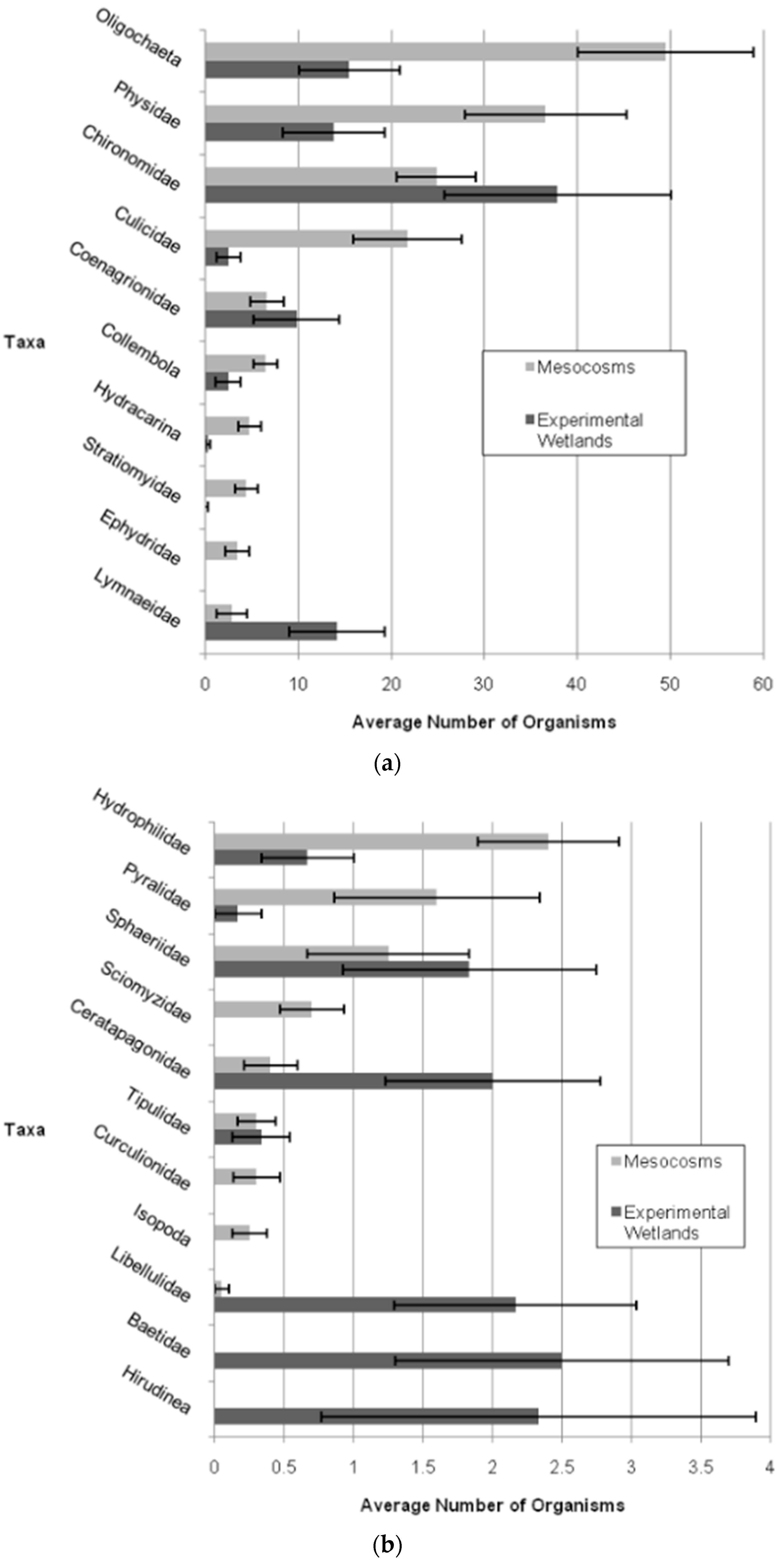
Hester–Dendy samples from the experimental wetlands had a higher average Shannon–Wiener diversity index (p < 0.05; t = 2.702; df = 44), N1 (p < 0.01; t = 3.220; df = 44), and taxa richness (p < 0.001; t = 5.279; df = 44), than did the mesocosms. The number of organisms for the mesocosms and experimental wetlands from the HD samples are presented in Figure 7. Analysis of the activity trap samples and the samples of organisms scraped from vegetation in the whole-ecosystem wetlands yielded no significant differences in macroinvertebrate populations between vegetation communities in the experimental wetlands.
Combining sample data from all sampling methods, a total of 33 taxa were collected from the experimental wetlands and the mesocosms—27 in the experimental wetlands and 23 in the mesocosms (Table 9 and Table 10). Ten taxa were not found in mesocosm samples that did appear in the experimental wetland samples. Six taxa were found in the mesocosms that were not found in the experimental wetlands.
When the sample size from each mesocosm was doubled to adjust for the difference in surface area between the Hester–Dendy traps in the mesocosms and those in the experimental wetlands, the average organism density by Hester–Dendy sample was higher in the mesocosms than in the experimental wetlands, (p < 0.05; t = 2.257; df = 30.870). In the activity trap samples, both taxa richness and organism density were higher in the mesocosms than in the experimental wetlands (p < 0.01; t = 2.801; df = 26), while E5 (a measure of evenness) was higher in the experimental wetlands than in the mesocosms (p < 0.05; t = 2.613; df = 14.340).
4. Discussion
4.1. Physicochemical Parameters
The data gathered using the YSI instrument indicated the harsh nature of the physical mesocosm environment, particularly with dissolved oxygen. On an average of at least six days during thirty-six days from late July to early September 2008, the average dissolved oxygen in the mesocosms in the morning dropped below 4 mg/L. On three of those days, it dropped below 3 mg/L. In Ohio, the minimum standard for dissolved oxygen in streams is 4.0.
With regard to hydrology, the deeper water seems to have resulted in more primary production. The DO in the deepest water reached both higher and lower levels, as well as accompanying higher diurnal DO changes, than did those in the shallowest mesocosms. This is a pattern that one would expect with higher productivity.
Unlike natural wetlands, the temperatures were not lower in the Typha spp. stands than they were in the mixed vegetation mesocosms. In natural stands of cattails, the density of the stems, combined with their height and width, create a swath of shade. In the mesocosms, sun hits the water from an angle at the edge, reducing the shading effect of the Typha stems, and the Typha stems were less dense than were the mixed vegetation stems. As a result, the mixed vegetation provided at least as much as shade as did the Typha.
The spacing between the Typha stems may have provided more space for the growth of filamentous algae than was available in the mixed vegetation mesocosms. This could have resulted in increased oxygen inputs via photosynthesis, resulting in slightly higher dissolved oxygen in the Typha as compared with the mixed vegetation mesocosms.
4.2. Effects of Hydrology on Macroinvertebrates
The hydrological regimes in this study do not reflect those in other studies nor likely those found in the natural environment. Deep water levels in this study were only 15–20 cm. These levels were considered drawdown levels in another study [24] and among the lowest water levels in another [21]. In addition, the pulsing mesocosms only received one significant pulse. Finally, to some degree, pump problems in the spring made all the mesocosms pulsing mesocosms, since there was considerable variability in flow across them all. Even so, there was one significant difference among mesocosms for macroinvertebrate diversity by hydrology, with mesocosms with high spring hydrology having higher diversity than two of the three other hydrologies.
This study’s results are consistent with those of Anderson and Smith [40], who found that playa marshes with wet winters have the highest diversity of macroinvertebrates. Similarly, Shummer et al. [21] found that a high spring hydrology yielded higher diversity when compared with steady state or high fall hydrologies. It is hypothesized that deeper water levels create a larger variety of habitats than do shallower ones, creating suitable conditions for a larger variety of organisms.
Other research regarding seasonal hydrology has indicated that a spring marsh drawdown yields increased macroinvertebrate densities, especially among midge larvae [3,41]. The results of this study are consistent with these results, with a much lower biomass of Chironomidae larvae being found in the high spring mesocosms as compared with mesocosms of all other hydrologies. The data from mesocosms that went dry in the spring confirm these findings, although they also indicate that such drawdowns can have a negative impact on gastropods, a significant organism in wetland environments.
Maintaining normal hydrology in Ohio wetlands—high water levels in the spring—appears to produce the highest level of macroinvertebrate diversity. However, employing a reverse hydrology—a spring drawdown—likely increases Chironomid productivity, serving as a useful tool for those seeking to provide food to migrating waterfowl that consume Chironomid larvae in the spring, although the negative impact on gastropods must also be taken into account.
Given the nature of the hydrological regimes in the mesocosms, the implications of this study are limited. In addition, macroinvertebrates were only collected at one point during the study. Chironomidae, in particular, typically have more than one generation during a season, and changes in hydrology could potentially shift the timing of those generations. The differences between the Chironomid mesocosm communities by hydrology could reflect differences in the timing of emergences rather than an overall difference in Chironomid productivity.
4.3. Macroinvertebrate Diversity in a Monoculture and in Mixed Vegetation
It was somewhat unexpected that there were no significant differences between diversity, evenness, or richness found between vegetation types in the Hester–Dendy samples, although in the literature, density, abundance, and biomass were often the parameters that differentiated macroinvertebrate populations from mixed vegetation and those from Typha monocultures rather than diversity.
The only significant difference between vegetation communities was produced by combining the samples from the separate mesocosms into a single sample, which indicated higher diversity in Typha mesocosms. This analytical step had the advantage of leveling out the patchy nature of macroinvertebrate distribution. It has the disadvantage of negating the value of using twenty replicates of an experimental condition.
The difference in diversity between the vegetation types was not linked to a difference in taxa richness. Batzer and Wissenger [3] noted that a variety of factors besides emergent macrophytes can affect macroinvertebrate populations, such as plant density and submersed plant communities. In studies of coastal wetlands of the upper Great Lakes, Gathman et al. [42] reinforced the complexity of the relationship between macrophytes and macroinvertebrates, noting that the effects of macrophyte density and submerged plants are not consistent.
The difference in diversity highlights the challenge of assessing biological diversity using mathematical formulae [43]. With regard to the Shannon–Wiener diversity index, given two samples with equal taxon richness and an equal distribution of organisms among taxa, any increase in the number of organisms in one taxon reduces the diversity index value. In this study, the difference in diversity indices between the vegetation conditions attained significance in one analysis, even though the taxa richness of the samples was equivalent and the minimum number of organisms in any given taxon was not significantly different between the two sets of samples.
The primary difference between the samples was in the number of Chironomids, with the samples from the mixed mesocosms containing significantly more Chironomids than those from the Typha mesocosms. From an ecological point of view, an increase in abundance in one or two taxa, particularly in a wetland sample, without a decrease in richness or in the number of organisms in any other given taxon would not seem to reflect a meaningful reduction in diversity. In other words, using the Shannon–Wiener index may cause one to overvalue samples with reasonable taxonomic diversity, evenness, and richness with limited productivity, as compared with samples with equivalent diversity, evenness, and richness with greater productivity.
The increase of diversity in macroinvertebrates with an increased diversity of wetland plants is commonly attributed to the variety of plant morphologies associated with plant diversity. While there is some difference in morphology among the emergent plants used in this study, all the vegetation was composed of single stems without any subsurface leaves or branches. The variation came in the size of the stems, the density of the growth habit, and to some degree, the stem shape.
While there were no significant differences based on vegetation differences, the difference in abundance between the two groups approached significance—averages of 100 organisms per mesocosm vs. 64. In addition, the biomass of chironomids in the mixed mesocosms was over 3× greater than that in the Typha spp. mesocosms. The diversity of organisms between vegetation treatments does not seem to have been significantly different, but the overall productivity may well have been.
As noted in the introduction, the release of allelochemicals from macrophytes could also play a role in differences in macroinvertebrate populations in the mesocosms [44]. Typha spp. are among the macrophytes identified as secreting allelochemicals [45]. The fact that fewer taxa were found on the surfaces of Typha spp. stems than were on the surfaces of the mixed vegetation would be consistent with this possibility.
4.4. Specific Macroinvertebrate Taxa and Vegetation
The data indicate that there were species-specific relationships between macroinvertebrates and vegetation. Hydrological conditions likely contributed to these differences, and some differences may reflect hydrologic differences alone. Vegetation density, floating vegetation (such as Lemna spp.), organism habitat requirements, organism food preferences, and inter-organism interaction all contribute to differences in taxa [41].
The significant differences between organism numbers by taxa and vegetation were for Coenagrionidae, Curculionidae, Culicidae, and Chironomidae. Coenagrionidae may be limited by the density of the stems in the mixed mesocosms, which would have restricted the movement of large flying insects. The absence of Anisoptera from all the mesocosm samples is consistent with the hypothesis that stem density may physically limit access to the mesocosms by large flying insects.
Orians and Wittenberger [46] provide indirect confirmation of the preference of Odonata for sites with lower vegetation density over those with high density, noting that female yellow-headed blackbirds settle in wetlands with more Odonata and that their choice of nesting site is inversely related to vegetation density. While some studies have linked larger insects with vegetation density [47,48], these studies were undertaken in settings with open water and fish. The former would give the larger insects access to the water, while predation by the latter would reduce large insect numbers in areas with low vegetation density.
Another factor in the difference in Zygoptera densities could be species preferences. Zygoptera have species-specific plant preferences for oviposition [49,50]. In addition, some do not oviposit on dead plants [51]. Mixed vegetation mesocosms seem to have contained more senescent plant material than did the Typha mesocosms.
Knight et al. [52] note that the density of macrophytes can significantly affect the presence of Culicidae larvae, with more larvae present in dense plant stands. This is consistent with the data indicating that more mosquitoes were present in the mixed than in the Typha mesocosms. However, Knight et al. [52] also provide a list, rating plants as to their predicted production of mosquitoes. According to this list, Typha has the highest rating for mosquito production, with Juncus having the lowest rating of the macrophytes used in this study. Collins and Resh [53] developed ratings based on four parameters: the intersection line value (an indicator of the menisci created when the plant stems break the water surface), crayfish food value, waterfowl food value, and fish obstruction value. Typha spp. were ranked as more mosquito-friendly than any of the three species in the mixed vegetation. The data in this study are not consistent with these ratings, recognizing that crayfish, waterfowl, and fish were not present in the mesocosms.
Other research has indicated mosquito densities vary considerably by species. Cx. erythrothorax has been positively associated with stem density [54], while two other species showed no vegetation preference. Studies have linked species to Eleocharis [55,56] and Carex spp. [57], species that are morphologically similar to Juncus effusus. Moquitoes have been positively associated with a species of Schoenoplectus [54] in preference to Typha spp. Anopheles albimanus was negatively associated with Typha, while An. vestitipennis was positively linked to Typha. On average, mosquitoes seem to prefer higher stem densities—a characteristic of the mixed vegetation mesocosms, with inter-species differences with regard to vegetation preferences.
Some Chironomidae used plants in the mixed mesocosms as a protective habitat. They were frequently found inside senescent Schoenoplectus stems (see below) but not in Typha stems, which suggests that mixed mesocosms may have provided a more diverse habitat for Chironomids than did Typha mesocosms. There were also differences in the rate of senescence among macrophytes, with Typha senescing later than either Sparganium or Schoenoplectus. Hargeby [58] noted that differences in the timing of senescence between submersed plants can affect macroinvertebrate populations.
4.5. Mesocosms and Whole-Ecosystem Wetlands
Despite the massive difference of scale and the dynamics associated with that difference, the physiochemical differences, as measured by a YSI instrument, between the mesocosms and the experimental wetlands are remarkably limited. The primary differences may be attributable to the increased amount of open water in the experimental wetlands. This increased surface area of exposed open water could increase the impact of solar radiation, which could result in increased water temperature and increased primary production, which could explain the higher temperatures, increased diurnal oxygen change (increased primary productivity), and increased pH (associated with primary productivity). This hypothesis is consistent with the nonsignificant differences between wetland 1 and wetland 2, in that wetland 1 likely receives more sun than does wetland 2, particularly afternoon sun.
Comparisons between the data collected in the whole-ecosystem wetlands and the mesocosms yielded mixed results. The increased diversity of habitats in the experimental wetlands, the depth of water, and the amount of open water compared to the mesocosms likely led to the differences between the two in macroinvertebrate diversity and richness. The presence of some open water has been identified as a particularly important feature for enhancing macroinvertebrate diversity [22,41]. The high stem density of vegetation in the mesocosms likely limited access by large flying insects (e.g., Aeshnidae) and may have been similarly inhospitable to rapidly swimming organisms like Dytiscidae and Haliplidae. Studies indicating increased prevalence of these taxa in dense vegetation [47,48] have been done in settings where open water and vertebrate predators were significant components of the overall environment. Water depth may have also played a role in the absence of Dytiscidae and Haliplidae. While Coleoptera have been found to prefer low water levels [59], Hyrophilidae appear best adapted to the lowest water levels and are the family of Coleoptera found in the mesocosms.
The absence of Baetidae and Caenidae might reflect any of a number of factors. Studies have linked the presence of Baetidae and/or Caenidae to pH and conductivity [60], water depth [59], DO concentrations [61], nutrient concentrations, and/or habitat heterogeneity [62] and vegetation [63]. Given that Baetidae and Caenidae prefer water depths the exceed those in the mesocosms, low water depths would seem to be the most likely reason that they do not appear in the mesocosms.
5. Conclusions
While it is not possible to make major generalizations based on this study, it can provide useful insights in the context of other research. For example, Typha spp. are particularly effective in reducing nutrient levels [64]. While this may make these species particularly useful in constructed wetlands designed to reduce nutrient levels, other research has indicated that monotypic Typha spp. stands are not as conducive to developing robust macroinvertebrate populations as are mixed vegetation wetlands.
In the face of or in anticipation of wetland dominance by Typha spp., efforts to maintain a diverse macrophyte community may not contribute to an increase in macroinvertebrate diversity (based on this study) but would likely contribute to an increase in macroinvertebrate density and biomass, particularly Chironomid biomass—a phenomenon previously identified by Kostecke [19]. This would suggest that wetlands with diverse emergent vegetation would provide more food for migrating waterfowl than would Typha spp. monocultures. Hence, the primary goal of a constructed wetland—nutrient reduction vs. habitat restoration—could impact the importance of limiting Typha.
In terms of hydrology, the study suggests that water levels below 20 cm are not deep enough to maintain the highest macroinvertebrate diversity. The impact of low hydrologies tend to be taxa-specific. Complete drawdowns seem to negatively impact Pulmonata, while it can have a positive effect on Chironomidae. This reinforces the value of spatial heterogeneity, reflected here in the varying water depths.
Finally, while the mesocosms in this study seemed to mimic the neighboring experimental wetlands (1 ha. each) in many ways, they lacked open water, vertebrate predators (e.g., fish and ducks), and many large invertebrate predators (e.g., crayfish, predacious beetles, almost all aquatic bugs, and dragonflies). Differences in scale likely had other impacts as well. Changing any of these factors to the system would have likely have a significant impact on the macroinvertebrate communities.
Supplementary Materials
The following supporting information can be downloaded at: https://www.mdpi.com/article/10.3390/land11091554/s1.
Funding
This research was partially supported by U.S. Environmental Protection Agency grant EM-83329801-0 (Olentangy River Wetland Research Park: Teaching, research and outreach) and by support provided by the Olentangy River Wetland Research Park and the Environmental Science Graduate Program at The Ohio State University.
Data Availability Statement
The data presented in this study are available in supplementary materials associated with this article: Data for Keljo Mesocosm Study.xls.
Acknowledgments
I am most grateful to individual faculty at The Ohio State University, Kenyon College, Kent State University and North Dakota State University, who provided input and support related to the project. I also very much appreciate the assistance and support of fellow graduate and undergraduate students at the Olentangy River Wetland Research Park.
Conflicts of Interest
The author declares no conflict of interest.
References
- Swanson, G.A.; Meyer, M.I.; Adomaitis, V.A. Foods consumed by breeding mallards on wetlands of South-Central North Dakota. J. Wildl. Manag. 1985, 49, 197–203. [Google Scholar] [CrossRef]
- Eldridge, J.L.; U.S. Fish and Wildlife Service. Waterfowl Management Handbook: Aquatic Invertebrates Important for Waterfowl Production. 13.3.3; U.S. Department of the Interior, Fish and Wildlife Service: Washington, DC, USA, 1990.
- Batzer, D.P.; Wissinger, S.A. Ecology of insect communities in nontidal wetlands. Annu. Rev. Entomol. 1996, 41, 75–100. [Google Scholar] [CrossRef] [PubMed]
- Piedade, M.T.F.; Parolin, P.; Junk, W.; Schöngart, J.; Wittmann, F.; Demarchi, L.O.; Lopes, A. Vegetation. In Fundamentals of Tropical Freshwater Wetlands; Dalu, T., Wasserman, R.J., Eds.; Elsevier: Amsterdam, The Netherlands, 2021; pp. 163–187. [Google Scholar]
- Papas, P. Effect of macrophytes on aquatic invertebrates—A literature review. In Technical Report Series; Arthur Rylah Institute for Environmental Research: Heidelberg, VIC, Australia, 2007; Volume 158, p. 29. [Google Scholar]
- Habib, S.; Yousuf, A.R. Effect of macrophytes on Phytophilous macroinvertebrate community: A review. J. Entomol. Zool. Stud. 2015, 3, 377–384. [Google Scholar]
- Hussain, Q.A.; Pandit, A.K. Macroinvertebrates in streams: A review of some ecological factors. Int. J. Fish. Aquac. 2012, 4, 114–123. [Google Scholar]
- Attrill, M.J.; Strong, J.A.; Rowden, A.A. Are Macroinvertebrate communities influenced by seagrass structural complexity? Ecography 2000, 23, 114–121. [Google Scholar] [CrossRef]
- Wilson, S.; Ricciardi, A. Epiphytic macroinvertebrate communities on Eurasian watermilfoil (Myriophyllum spicatum) and native milfoils Myriophyllum sibericum and Myriophyllum alterniflorum in eastern North America. Can. J. Fish. Aquat. Sci. 2009, 66, 18–30. [Google Scholar] [CrossRef]
- Batzer, D.P.; Resh, V.H. Trophic Interactions among a beetle predator, a chironomid grazer, and periphyton in a seasonal wetland. Oikos 1991, 60, 251–257. [Google Scholar] [CrossRef]
- Mabidi, A.; Bird, M.S.; Perissinotto, R. Relationships between vegetation cover (Schoenoplectus decipiens) and wetland macroinvertebrate assemblages in a semi-arid landscape (Eastern Cape Karoo, South Africa). Hydrobiologia 2020, 847, 2049–2064. [Google Scholar] [CrossRef]
- Buxton, M.; Cuthbert, R.N.; Dalu, T.; Nyamukondiwa, C.; Wasserman, R.J. Predator density modifies mosquito regulation in increasingly complex environments. Pest Manag. Sci. 2020, 76, 2079–2086. [Google Scholar] [CrossRef]
- Phiri, C.; Chakona, A.; Day, J.A. The effect of plant density on epiphytic macroinvertebrates associated with a submerged macrophyte, Lagarosiphon ilicifolius Obermeyer, in Lake Kariba, Zimbabwe. Afr. J. Aquat. Sci. 2011, 36, 289–297. [Google Scholar] [CrossRef]
- Smock, L.A.; Stoneburner, D.L. The response of macroinvertebrates to aquatic macrophyte decomposition. Oikos 1980, 35, 397–403. [Google Scholar] [CrossRef]
- Keast, A. The introduced aquatic Myriophyllum spicatum as habitat for fish and their invertebrate prey. Can. J. Zool. 1984, 62, 1289–1303. [Google Scholar] [CrossRef]
- Hanson, J.M. Macroinvertebrate size-distributions of two contrasting freshwater macrophyte communities. Freshw. Biol. 1990, 24, 481–491. [Google Scholar] [CrossRef]
- Meyer, M.D.; Davis, C.A.; Dvorett, D. Response of wetland invertebrate communities to local and landscape factors in North Central Oklahoma. Wetlands 2015, 35, 533–546. [Google Scholar] [CrossRef]
- Whatley, M.; Loon, E.; Vonk, J.; Geest, H.; Admiraal, W. The role of emergent vegetation in structuring aquatic insect communities in peatland drainage ditches. Aquat. Ecol. 2014, 48, 267–283. [Google Scholar] [CrossRef]
- Kostecke, R.M.; Smith, L.M.; Hands, H.M. Macroinvertebrate response to cattail management at Cheyenne Bottoms, Kansas, USA. Wetlands 2005, 25, 758–763. [Google Scholar] [CrossRef]
- Kulesza, A.E.; Holomuzki, J.R.; Klarer, D.M. Benthic community structure in stands of Typha angustifolia and herbicide-treated and untreated Phragmites australis. Wetlands 2008, 28, 40–56. [Google Scholar] [CrossRef]
- Schummer, M.L.; Eason, K.M.; Hodges, T.J.; Farley, E.B.; Sime, K.R.; Coluccy, J.M.; Tozer, D.C. Response of aquatic macroinvertebrate density and diversity to wetland management and structure in the Montezuma Wetlands Complex, New York. J. Great Lakes Res. 2021, 47, 875–883. [Google Scholar] [CrossRef]
- Schummer, M.L.; Palframan, J.; McNaughton, E.; Barney, T.; Petrie, S.A. Comparisons of bird, aquatic macroinvertebrate, and plant communities among dredged ponds and natural wetland habitats at Long Point, Lake Erie, Ontario. Wetlands 2012, 32, 945–953. [Google Scholar] [CrossRef]
- Lawrence, B.A.; Bourke, K.; Lishawa, S.C.; Tuchman, N.C. Typha invasion associated with reduced aquatic macroinvertebrate abundance in northern Lake Huron coastal wetlands. J. Great Lakes Res. 2016, 42, 1412–1419. [Google Scholar] [CrossRef]
- Riley, T.Z.; Bookhout, T.A. Response of aquatic macroinvertebrates to early-spring drawdown in nodding smartweed marshes. Wetlands 1990, 10, 173–185. [Google Scholar] [CrossRef]
- de Szalay, F.A.; Carroll, L.C.; Beam, J.A.; Resh, V.H. Temporal overlap of nesting duck and aquatic invertebrate abundances in the grasslands ecological area, California, USA. Wetlands 2003, 23, 739–749. [Google Scholar] [CrossRef]
- Robinson, C.T.; Uehlinger, U.; Monaghan, M.T. Effects of a multi-year experimental flood regime on macroinvertebrates downstream of a reservoir. Aquat. Sci. 2003, 65, 210–222. [Google Scholar] [CrossRef]
- Whiles, M.R.; Goldowitz, B.S. Macroinvertebrate communities in central platte river wetlands: Patterns across a hydrologic gradient. Wetlands 2005, 25, 462–472. [Google Scholar] [CrossRef]
- Caiazza, M.K.; Nieset, J.E.; Romito, A.; Szalay, F.A. Plant and invertebrate community changes caused by flood-pulsing in a constructed riparian wetland. In Proceedings of the American Geophysical Union, Spring Meeting, New Orleans, LA, USA, 1 May 2005. [Google Scholar]
- Batzer, D.P. The seemingly intractable ecological responses of invertebrates in North American Wetlands: A review. Wetlands 2013, 33, 1–15. [Google Scholar] [CrossRef]
- Mitsch, W.J. Wetland creation, restoration, and conservation: A Wetland Invitational at the Olentangy River Wetland Research Park. Ecol. Eng. 2005, 24, 243–251. [Google Scholar] [CrossRef]
- Merritt, R.W.; Cummins, K.W. An Introduction to the Aquatic Insects of North America; Kendall/Hall Publishing: Dubuque, IA, USA, 1996; p. 862. [Google Scholar]
- Benke, A.C.; Huryn, A.D.; Smock, L.A.; Wallace, J.B. Length-mass relationships for freshwater macroinvertebrates in North America with particular reference to the southeastern united states. J. N. Am. Benthol. Soc. 1999, 18, 308–343. [Google Scholar] [CrossRef]
- Cummins, K.W.; Wilzbach, M.; Kolouch, B.; Merritt, R. Estimating macroinvertebrate biomass for stream ecosystem assessments. Int. J. Environ. Res. Public Health 2022, 19, 3240. [Google Scholar] [CrossRef]
- Spieles, D.J.; Mitsch, W.J. Macroinvertebrate community structure in high- and low-nutrient constructed wetlands. Wetlands 2000, 20, 716–729. [Google Scholar] [CrossRef]
- Gamble, D.L.; Washburn, S.W.; Mitsch, W.J. Macroinvertebrate abundance and diversity in two ten-year-old created wetland ecosystems. In Olentangy River Wetland Research Park at The Ohio State University Annual Report 2004; Mitsch, W.J., Zhang, L., Altor, A.E., Mitsch, W.J., Zhang, L., Altor, A.E., Eds.; The Ohio State University: Columbus, OH, USA, 2005; p. 200. [Google Scholar]
- Simpson, E.H. Measurement of diversity. Nature 1949, 163, 688. [Google Scholar] [CrossRef]
- Shannon, C.E. A mathematical theory of communication. Bell Syst. Tech. J. 1948, 27, 379–423. [Google Scholar] [CrossRef]
- Hill, M.O. Diversity and evenness: A unifying notation and its consequences. Ecology 1973, 54, 427–432. [Google Scholar] [CrossRef] [Green Version]
- Molinari, J. A calibrated index for the measurement of evenness. Oikos 1989, 56, 319–326. [Google Scholar] [CrossRef]
- Anderson, J.T.; Smith, L.M. Invertebrate response to moist-soil management of playa wetlands. Ecol. Appl. 2000, 10, 550–558. [Google Scholar] [CrossRef]
- Batzer, D.P.; Cooper, R.; Wissinger, S.A. Wetland animal ecology. In Ecology of Freshwater and Estuarine Wetlands; Batzer, D.P., Sharitz, R.R., Eds.; University of California Press: Oakland, CA, USA, 2006; pp. 151–184. [Google Scholar]
- Gathman, J.P.; Burton, T.M.; Armitage, B.J. Coastal wetlands of the upper great lakes: Distribution of invertebrate communities in response to environmental variation. In Invertebrates in Freshwater Wetlands of North America; Batzer, D.P., Rader, R.B.A., Wissinger, S.A., Eds.; John Wiley and Sons: New York, NY, USA, 1999; p. 1100. [Google Scholar]
- Barrantes, G.; Sandoval, L. Conceptual and statistical problems associated with the use of diversity indices in ecology. Rev. Biol. Trop. 2009, 57, 451–460. [Google Scholar] [CrossRef]
- Habib, S.; Yousuf, A.R. Phytophilous macroinvertebrate community of an eutrophic lake in Kashmir Himalayas. J. Entom. Zool. Stud. 2016, 4, 318–325. [Google Scholar]
- Jarchow, M.E.; Cook, B.J. Allelopathy as a mechanism for the invasion of Typha angustifolia. Plant Ecol. 2009, 204, 113–124. [Google Scholar] [CrossRef]
- Orians, G.H.; Wittenberger, J.F. Spatial and temporal scales in habitat selection. Am. Nat. 1991, 137, S29–S49. [Google Scholar] [CrossRef]
- Armstrong, D.P.; Nudds, T.D. Factors influencing invertebrate size distributions in prairie potholes and implications for coexisting duck species. Freshw. Invertebr. Biol. 1985, 4, 41–47. [Google Scholar] [CrossRef]
- Tolonen, K.T.; Hämäläinen, H.; Holopainen, I.J.; Mikkonen, K.; Karjalainen, J. Body size and substrate association of littoral insects in relation to vegetation structure. Hydrobiologia 2003, 499, 179–190. [Google Scholar] [CrossRef]
- Martens, A. Initial preference of oviposition sites: Discrimination between living and dead plant material in Sympecma fusca and Coenagrion caerulescens (Odonata: Lestidae, Coenagrionidae). EJE 2001, 98, 121–123. [Google Scholar] [CrossRef]
- Lambret, P.; Besnard, A.; Matushkina, N. Plant preference during oviposition in the endangered dragonfly Lestes macrostigma (Odonata: Zygoptera) and consequences for its conservation. J. Insect Conserv. 2015, 19, 741–752. [Google Scholar] [CrossRef]
- Thaokar, N.R.; Verma, P.R.; Andrew, R.J. Breeding behaviour of the Coromandel Marsh Dart Damselfly (Zygoptera:Coenagrionidae: Ceriagrioncoromandelianum (Fabricius)) in central India. J. Threat. Taxa 2018, 10, 11443–11449. [Google Scholar] [CrossRef]
- Knight, R.L.; Walton, W.E.; O’Meara, G.F.; Reisen, W.K.; Wass, R. Strategies for effective mosquito control in constructed treatment wetlands. Ecol. Eng. 2003, 21, 211–232. [Google Scholar] [CrossRef]
- Collins, J.N.; Resh, V.H. Guidelines for the Ecological Control of Mosquitoes in Non-tidal Wetlands of the San Francisco Bay Area; Mosquito Vector Control Association, Inc.; University of California Mosquito Research Program: Sacramento, CA, USA, 1989; p. 93. [Google Scholar]
- Metzger, M.E. A legacy of mosquito control through wetland management: A tribute to William E. Walton and his contributions to science and entomology. Wetl. Ecol. Manag. 2021. [Google Scholar] [CrossRef]
- Rejmankova, E.; Roberts, D.R.; Harbach, R.E.; Pecor, J.; Peyton, E.L.; Manguin, S.; Krieg, R.; Polanco, J.; Legters, L. Environmental and regional determinants of anopheles (Diptera: Culicidae) larval distribution in Belize, Central America. Environ. Entomol. 1993, 22, 978–992. [Google Scholar] [CrossRef]
- Grieco, J.P.; Johnson, S.; Achee, N.L.; Masuoka, P.; Pope, K.; Rejmánková, E.K.; Vanzie, E.; Andre, R.; Roberts, D. Distribution of Anopheles albimanus, Anopheles vestitipennis, and Anopheles crucians associated with land use in Northern Belize. J. Med. Entomol. 2006, 43, 614–622. [Google Scholar] [CrossRef]
- Lewis, D.J.; Bennett, G.F. Observations on the biology of Mansonia perturbans (Walker) (Diptera: Culicidae) in the Nova Scotia–New Brunswick border region. Can. J. Zool. 1980, 58, 2084–2088. [Google Scholar] [CrossRef]
- Hargeby, A. Macrophyte associated invertebrates and the effect of habitat permanence. Oikos 1990, 57, 338–346. [Google Scholar] [CrossRef]
- Shrestha, S.; Shah, R.D.T.; Doody, T.; Cuddy, S.; Shah, D.N. Establishing the relationship between benthic macroinvertebrates and water level fluctuation in subtropical shallow wetlands. Environ. Monit. Assess. 2021, 193, 534. [Google Scholar] [CrossRef]
- Gezie, A.; Mulat, W.L.; Anteneh, W.; Dejen, E.; Kloos, H.; Mereta, S.T. Habitat Suitability modelling of benthic macroinvertebrate community in Wetlands of Lake Tana Watershed, Northwest Ethiopia. Wetlands 2020, 40, 853–864. [Google Scholar] [CrossRef]
- Armendáriz, L.C.; Cortese, B.; Rodriguez, M.; Capítulo, A.R. Ecosystem services of runoff marshes in urban lowland basins: Proposals for their management and conservation. Knowl. Manag. Aquat. Ecosyst. 2017, 418, 12. [Google Scholar] [CrossRef]
- Sartori, L.; Canobbio, S.; Cabrini, R.; Fornaroli, R.; Mezzanotte, V. Macroinvertebrate assemblages and biodiversity levels: Ecological role of constructed wetlands and artificial ponds in a natural park. J. Limnol. 2014, 73. [Google Scholar] [CrossRef] [Green Version]
- Batzer, D.P.; Taylor, B.E.; DeBiase, A.E.; Brantley, S.E.; Schultheis, R. Response of aquatic invertebrates to ecological rehabilitation of southeastern USA depressional wetlands. Wetlands 2015, 35, 803–813. [Google Scholar] [CrossRef]
- Bansal, S.; Lishawa, S.C.; Newman, S.; Tangen, B.A.; Wilcox, D.; Albert, D.; Anteau, M.J.; Chimney, M.J.; Cressey, R.L.; DeKeyser, E.; et al. Typha (Cattail) Invasion in North American Wetlands: Biology, Regional Problems, Impacts, Ecosystem Services, and Management. Wetlands 2019, 39, 645–684. [Google Scholar] [CrossRef] [Green Version]
Figure 1.
The site and mesocosm schematics: (a) an aerial schematic of the site; (b) a cross-section of a mesocosm, which illustrates the two drainage configurations; (c) a schematic of a mixed vegetation mesocosm from above. Each mesocosm is approximately 1 m2.
Figure 1.
The site and mesocosm schematics: (a) an aerial schematic of the site; (b) a cross-section of a mesocosm, which illustrates the two drainage configurations; (c) a schematic of a mixed vegetation mesocosm from above. Each mesocosm is approximately 1 m2.

Figure 2.
Average water depth (±standard error) in 2008 by mesocosm type: (a) by hydrologic regime and season; (b) by season for high spring and high fall.
Figure 2.
Average water depth (±standard error) in 2008 by mesocosm type: (a) by hydrologic regime and season; (b) by season for high spring and high fall.

Figure 3.
Shannon–Wiener macroinvertebrate diversity indices for aggregated data for vegetation and hydrology treatment types, using Hutcheson t-tests (significant differences a > b, b > c, d > e, f; + d-e = n.s. within Typha mesocosms).
Figure 3.
Shannon–Wiener macroinvertebrate diversity indices for aggregated data for vegetation and hydrology treatment types, using Hutcheson t-tests (significant differences a > b, b > c, d > e, f; + d-e = n.s. within Typha mesocosms).

Figure 4.
HD samples: the number of taxa (±standard error) found approaches significance by mesocosm type (p < 0.10; t = −1.97; df = 38).
Figure 4.
HD samples: the number of taxa (±standard error) found approaches significance by mesocosm type (p < 0.10; t = −1.97; df = 38).

Figure 5.
Epiphytic samples: (a) the number of taxa found (±standard error) compared is significantly different between mesocosm type (n = 8, p < 0.05); (b) number of epiphytic samples with a given taxon present by mesocosm type.
Figure 5.
Epiphytic samples: (a) the number of taxa found (±standard error) compared is significantly different between mesocosm type (n = 8, p < 0.05); (b) number of epiphytic samples with a given taxon present by mesocosm type.

Figure 6.
Average number of organisms by taxa by vegetation with standard error lines.

Figure 7.
Average number of organisms by taxa in Hester–Dendy samples from the experimental wetlands and the mesocosms in 2008 (mesocosm sample size adjusted to reflect differences in surface area between traps used in the mesocosms and those used in the experimental wetlands). (a) High frequency taxa; (b) middle frequency taxa, (c) low frequency taxa.


Table 1.
The average number (±standard error) of organisms by taxa in reserved subsamples used to seed mesocosms in July 2007.
Table 1.
The average number (±standard error) of organisms by taxa in reserved subsamples used to seed mesocosms in July 2007.
| Taxa | Avg. Number of Organisms per Sample |
|---|---|
| Oligochaeta | 12.29 ± 2.63 (n = 7) |
| Physidae | 22.71 ± 3.13 (n = 7) |
| Lymnaeidae | 2.14 ± 0.40 (n = 7) |
| Planorbidae | 1.00 ± 0.44 (n = 7) |
| Corbiculidae | 0.14 ± 0.14 (n = 7) |
| Sphaeriidae | 7.29 ± 1.70 (n = 7) |
| Hydracarina | 0.71 ± 0.36 (n = 7) |
| Caenidae * | 0.14 ± 0.14 (n = 7) |
| Coenagrionidae | 2.57 ± 0.53 (n = 7) |
| Libellulidae | 0.14 ± 0.14 (n = 7) |
| Dytiscidae * | 0.71 ± 0.29 (n = 7) |
| Haliplidae * | 0.29 ± 0.29 (n = 7) |
| Pyralidae | 0.14 ± 0.14 (n = 7) |
| Ceratapagonidae | 0.43 ± 0.20 (n = 7) |
| Chironomidae | 11.57 ± 1.49 (n = 7) |
| Ephydridae | 2.00 ± 0.87 (n = 7) |
*—Taxa not found in final samples from mesocosms.
Table 2.
Significant differences between YSI parameters by mesocosm vegetation type.
| Vegetation and YSI Parameters | ||||||
|---|---|---|---|---|---|---|
| DO AM | DO PM | DO Avg. | DO Min. Avg. | DO Max. Avg. | DO Diurnal | |
| Mixed | 4.0 *** | 5.1 *** | 4.5 **** | 2.3 | 7.7 ** | 0.8 *** |
| Typha | 4.5 *** | 7.2 *** | 5.6 **** | 2.4 | 11.2 ** | 2.7 *** |
| Cond PM | Cond Avg. | Cond Diurnal | ||||
| Mixed | 628.4 | 634.5 ** | 630.30 | 8.3 **** | ||
| Typha | 635.8 | 623.0 ** | 630.55 | −17.9 **** | ||
n = 40, ** p < 0.01, *** p < 0.001, **** p < 0.0001.
Table 3.
Significant differences between YSI parameters by mesocosm hydrology type.
| Hydrology and YSI Parameters | |||
|---|---|---|---|
| Temperature Avg. | Temperature AM | ||
| HF | 23.4 | 21.7 | |
| HS | 23.5 a | 22.0 a | |
| P | 23.0 c | 21.4 b | |
| S | 23.4 | 21.6 c | |
| DO Min. | DO Max. | DO Diurnal | |
| HF | 2.2 d | 12.4 f | 2.9 h |
| HS | 2.8 e | 7.7 g | 0.7 i |
| P | 2.4 | 9.2 | 1.9 |
| S | 2.2 d | 8.5 | 1.3 |
| Cond Avg. | Cond AM | Cond PM | |
| HF | 647.6 j | 648.6 j | 646.2 k |
| HS | 608.5 k | 613.9 k | 603.9 l |
| P | 635.6 l | 638.5 l | 638.8 |
| S | 638.0 l | 641.2 m | 632.4 |
n = 40, a–c p < 0.05, a–b p < 0.001. n = 40, f–g p < 0.10, h–i p < 0.05, d–r p < 0.01. n = 40, k–l p < 0.05, k–m p < 0.01, j–k p < 0.001.
Table 4.
Significant differences between YSI parameters by mesocosm hydrology type and vegetation type.
Table 4.
Significant differences between YSI parameters by mesocosm hydrology type and vegetation type.
| Hydrology by Vegetation and YSI Parameters | ||||
|---|---|---|---|---|
| Mixed | Temperature AM | |||
| HF | 21.8 | |||
| HS | 22.2 a | |||
| P | 21.5 b | |||
| S | 21.6 c | |||
| Typha | DO Avg. | DO Max. | DO PM | DO Diurnal |
| HF | 6.8 d | 17.3 d | 9.9 d | 5.2 d |
| HS | 5.2 e | 8.7 f | 5.9 f | 1.3 f |
| P | 5.5 | 9.8 e | 6.9 e | 2.2 e |
| S | 5.2 e | 10.5 e | 6.6 e | 2.2 e |
| Typha | Cond Avg. | Cond PM | ||
| HF | 637.2 h | 646.6 h | ||
| HS | 608.4 g | 605.8 g | ||
| P | 638.3 h | 641.1 h | ||
| S | 638.0 h | 650.8 i | ||
n = 20, a–c p < 0.05, a–b p < 0.01. n = 20, d–e p < 0.05, d–f p < 0.01. n = 20, g–h p < 0.05, g–i p < 0.01.
Table 5.
Mean macrophyte stem counts (±standard error) in November 2008 by vegetation treatment in mesocosms.
Table 5.
Mean macrophyte stem counts (±standard error) in November 2008 by vegetation treatment in mesocosms.
| Species | Typha Mesocosms | Mixed Mesocosms |
|---|---|---|
| Typha spp. | 103 ± 5.00 | 2.7 ± 1.3 |
| Sparganium eurycarpum | 0 | 36.9 ± 4.1 |
| Schoenoplectus tabernaemontani | 0 | 201 ± 23 |
| Juncus effusus | 0 | 1046 ± 160 |
| Other | 16.5 ± 12.1 + | 0.55 ± 0.46 |
+ 99% of these stems were found in two mesocosms (328 stems), distributed between two hydrologies.
Table 6.
Diversity indices by hydrology and vegetation.
| Hydrology and Diversity | |||
|---|---|---|---|
| Typha | Shannon–Wiener | Simpson | Hill’s |
| HF | 1.3 b | 3.1 b | 3.8 c |
| HS | 1.7 a | 4.7 a | 5.5 a |
| P | 1.3 b | 3.2 b | 3.8 c |
| S | 1.5 | 3.6 | 4.4 |
| Mixed | Shannon–Wiener | Simpson | Hill’s |
| HF | 1.4 d | 3.4 | 4.1 d |
| HS | 1.7 c | 4.8 c | 5.8 c |
| P | 1.3 d | 2.7 d | 3.6 d |
| S | 1.5 | 3.7 | 4.4 |
a–b p < 0.05, a–c p < 0.01. n = 40, c–d p < 0.05.
Table 7.
Average number of organisms by taxa in all mesocosms that were affected by dry and wet conditions by month in 2008.
Table 7.
Average number of organisms by taxa in all mesocosms that were affected by dry and wet conditions by month in 2008.
| Taxon | Hydrology by Month | February | March | April |
|---|---|---|---|---|
| Physidae | Dry | 7.00 * | 6.82 * | 4.50 * |
| Not dry | 25.04 * | 22.62 * | 22.87 * | |
| Hydracarina | Dry | 0.93 * | 1 | 1.1 |
| Not dry | 3.28 * | 2.93 | 2.83 | |
| Chironomidae | Dry | 17.53 * | 17.91 | 19.6 |
| Not dry | 9.36 * | 10.34 | 10.03 |
n = 40, * p < 0.05.
Table 8.
The number of taxa found in samples by sample type and sample location.
| Experimental Wetland and Mesocosm YSI Parameters Compared | ||
|---|---|---|
| Temperature PM | Temperature Diurnal | |
| M | 25.5 b | 3.8 d |
| T | 25.7 b | 4.1 d |
| Outflow W1 | 27.5 a | 9.4 a |
| Outflow W2 | 26.0 | 6.9 c |
| EW Avg | 26.7 | 8.2 e |
| DO Diurnal | ||
| M | 0.8 g | |
| T | 2.7 h | |
| Outflow W1 | 8.8 f | |
| Outflow W2 | 4.1 | |
| EW Avg | 6.4 i | |
| pH Avg. | pH PM | |
| M | 7.0 k | 7.0 l |
| T | 7.2 | 7.3 k |
| Outflow W1 | 8.4 j | 9.2 j |
| Outflow W2 | 8.2 | 8.6 |
| EW Avg | 8.2 | 8.9 m |
n = 43, a–b p < 0.05, a–c p < 0.01, a–d, b–d, d–e p < 0.0001. n = 42, f–h, h–i p < 0.01, f–g p < 0.0001. n = 43, j–k, k–m p < 0.05, j–l p < 0.01.
Table 9.
The number of taxa found in samples by sample type and sample location.
| Sample Type | Experimental Wetlands | Mesocosms | Total |
|---|---|---|---|
| Hester–Dendy | 23 (n = 6) | 22 (n = 40) | 29 |
| Activity Trap | 21 (n = 12) | 17 (n = 12) | 28 |
| Vegetation Surface | 20 (n = 13) | 15 (n = 12) | 23 |
| Total Taxa | 27 | 23 | 33 |
Table 10.
Taxa appearing in Hester–Dendy (HD), dip net (mesocosm seed sub-samples), activity trap (AT), and vegetation surface (VS) samples by year and location (EW—experimental wetlands, MES—mesocosms).
Table 10.
Taxa appearing in Hester–Dendy (HD), dip net (mesocosm seed sub-samples), activity trap (AT), and vegetation surface (VS) samples by year and location (EW—experimental wetlands, MES—mesocosms).
| Year | 2008 | |||||
|---|---|---|---|---|---|---|
| Sample Type | HD | AT | VS | |||
| Location | EW | MES | EW | MES | EW | MES |
| Taxon | ||||||
| Horsehair Worm (Nematomorpha) | X | |||||
| Leech (Hirudinea) | X | |||||
| Aquatic Worm (Oligochaeta) | X | X | X | X | X | X |
| Apple Snail (Viviparidae) | X | |||||
| Physid Snail (Physidae) | X | X | X | X | X | X |
| Lymnaeid Snail (Lymnaeidae) | X | X | X | X | X | X |
| Planorbid Snail (Planorbidae) | X | |||||
| Asian Clam (Corbicula fluminea) | X | X | X | |||
| Fingernail Clam (Sphaeriidae) | X | X | X | X | X | |
| Aquatic Sow Bug (Isopoda) | X | X | X | |||
| Scud (Amphipoda) | X | X | ||||
| Water Mite (Hydracarina) | X | X | X | X | ||
| Springtail (Collembola) | X | X | X | X | X | |
| Small Minnow Mayfly (Baetidae) | X | X | X | |||
| Small Squaregill Mayfly (Caenidae) | X | X | X | |||
| Damselfly (Coenagrionidae) | X | X | X | X | X | X |
| Dragonfly (Aeshnidae) | X | X | X | |||
| Dragonfly (Libellulidae) | X | X | X | X | ||
| True Bug (Hemiptera) | X | X | ||||
| Water Scavenger Beetle (Hydrophilidae) | X | X | X | X | X | X |
| Predaceous Diving Beetle (Dytiscidae | X | X | X | |||
| Crawling Water Beetle (Haliplidae) | X | X | X | |||
| Weevil (Curculionidae) | X | |||||
| Minute Moss Beetle (Hydraenidae) | X | X | ||||
| Moth (Pyralidae) | X | X | X | X | X | X |
| Marsh Fly (Sciomyzidae) | X | X | ||||
| Biting Midge (Ceratapagonidae) | X | X | X | |||
| Crane Fly (Tipulidae) | X | X | X | X | X | X |
| Mosquito (Culicidae) | X | X | X | X | X | X |
| Midge (Chironomidae) | X | X | X | X | X | X |
| Soldier Fly (Stratiomyidae) | X | X | X | X | ||
| Shore Fly (Ephydridae) | X | X | X | |||
| Flower Fly (Syrphidae) | X | |||||
Publisher’s Note: MDPI stays neutral with regard to jurisdictional claims in published maps and institutional affiliations. |
© 2022 by the author. Licensee MDPI, Basel, Switzerland. This article is an open access article distributed under the terms and conditions of the Creative Commons Attribution (CC BY) license (https://creativecommons.org/licenses/by/4.0/).
Share and Cite
MDPI and ACS Style
Keljo, K.S. Effects of Hydrologic Pulsing and Vegetation on Invertebrate Communities in Wetlands. Land 2022, 11, 1554. https://doi.org/10.3390/land11091554
AMA Style
Keljo KS. Effects of Hydrologic Pulsing and Vegetation on Invertebrate Communities in Wetlands. Land. 2022; 11(9):1554. https://doi.org/10.3390/land11091554
Chicago/Turabian StyleKeljo, Kurt S. 2022. "Effects of Hydrologic Pulsing and Vegetation on Invertebrate Communities in Wetlands" Land 11, no. 9: 1554. https://doi.org/10.3390/land11091554
Note that from the first issue of 2016, this journal uses article numbers instead of page numbers. See further details here.