
Mapping Floristic Composition Using Sentinel-2A and a Case Study Evaluation of Its Application in Elephant Movement Ecology in Sagalla, Kenya
1
Save the Elephants, P.O. Box 54667, Nairobi 00200, Kenya
2
Department of Zoology, University of Oxford, Oxford OX1 3SZ, UK
*
Author to whom correspondence should be addressed.
Remote Sens. 2022, 14(21), 5386; https://doi.org/10.3390/rs14215386
Submission received: 31 July 2022
/
Revised: 18 October 2022
/
Accepted: 19 October 2022
/
Published: 27 October 2022
(This article belongs to the Special Issue Landscape Ecology in Remote Sensing)
Abstract
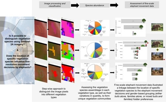
:The quantification of vegetation structure and composition at local and global scales provides valuable information for understanding the balance of the natural and human-made environment, which is crucial for natural resource planning and management, and the sustenance of ecosystem biodiversity. In this study, we proposed using the Sentinel 2A imagery to classify vegetation cover into communities based on the floristic association of individual vegetation species. We apply traditional remote sensing techniques to process the satellite image and identify training regions of interest (ROI) which are thoroughly assessed for spectral uniqueness before using the pixel-based supervised classification algorithms for our classification. Ground truthing assessment and species dominance computations are done to determine the vegetation community composition and naming based on floristic associations. We apply the floristic compositions output in analysing elephant movement tracks in the area, to assess the potential influence the location of specific vegetation species and communities utilized by elephants has on their movement and presence, as well as on elephant bulls and family groupings. The results show that the 10 m spatial resolution Sentinel-2A is suitable for investigating and mapping vegetation species in communities for large-scale mapping operations. We determined Near-Infrared band 8 and shortwave Infrared band 11 as key for identifying and differentiating ROIs at the floristic association community vegetation mapping level. We attained an overall accuracy of 87.395%. The analysis proved the 10 m spatial resolution of Sentinel 2A to be sufficient in distinguishing vegetation communities, including those with similar dominant species but variations in other contributing species. We also found a direct connection between vegetation location and elephant movement based on the summative analysis of utilised vegetation by the different elephant groupings. Bull elephants were predominantly present in areas with Combretum, family groups in areas with Commiphora, and mixed groups with both bulls and families in areas with Commiphora, and Cissus. This study shows the value that remote-sensing scientific support can offer conservationists and governments in objective evidence-based land management, policy making and governance.
1. Introduction
Historically, elephants and humans have been integral players in the structuring of the African savanna landscape [1]. However, this has dramatically changed in recent times, with human practices playing a more significant role as the dominant disruptive agents with unforeseen consequences to the ecosystem and biodiversity function [2]. Increasing human populations have resulted in the rapid expansion of human infrastructure in road networks, settlements, and cultivated fields into previously wildlife natural habitats. Consequently, there has been increasing loss of natural wildlife habitat, compromised landscape connectivity, degraded natural fodder and ultimately, the elephant populations have significantly declined in relation to their historical ranges and sizes [3,4]. As their natural habitat diminishes, elephants and people are progressively in closer contact with each other, resulting in what is termed Human-Elephant Conflict (HEC) [5]. HEC constitutes conflict over shared resources and space, and has detrimental consequences of crop raiding and destruction, and, in extreme instances, loss of life [6,7,8,9,10]. Continued landscape transformations by the increasing human populations pushes elephants and humans to live in closer proximity, thereby contributing to increased conflict cases, with significant fatal incidences [5]. In Kenya alone, it is reported that 100 problem elephants on average are shot by wildlife authorities, and about 200 cases were reported of elephant conflict related deaths between 2010 and 2017 [11]. The intensity of crop-raiding in farmland areas within 5 km from national parks’ and protected areas’ boundaries has been on the rise since 2014 [12] as a result of increased drought periods and reduced rainfall which lowers the quality of natural forage, hence making crops, at all growth stages, the next likely fodder option [13,14,15,16]. Studies conducted in two regions of varying vegetative climatic conditions showed significant economic losses to crop-raiding elephants; 414 farmers in the semi-arid areas around the Marsabit National Park and Reserve made loses amounting to USD 208,814 within the period of a year, between August 2004 and July 2005 [17], averaging about USD 500 per farmer, while their counterparts farming in the highland areas bordering Meru National Park incurred more loses to the tune of USD 120,308 amongst 144 farmers, averaging at USD 835 per farmer within a similar one-year time frame, between August 2010 and July 2011 [18]. Conflict in other parts of the world is documented in Sri Lanka, which is home to approximately 3000 elephants, and documents over 200 elephant and 70 human mortalities annually from human-elephant conflict [19,20]. In India, the deaths of 100 elephants and 400 humans have been recorded as a result of conflict incidences, as well as direct afflictions to over 500,000 families as a result of crop-raiding [21]. HEC has become a considerable threat to the conservation of biodiversity, and thus it is the goal of afflicted countries to manage this conflict. There has been considerable growth in the understanding of elephant behavior, as well as the spatial-temporal patterns of HEC, and this has in turn lead to the proposal, development, implementation and reproduction of a wide array of deterrence and mitigation approaches [13,22,23,24,25].
Kenya presents common conflict instances between elephants that are free-ranging and farmers. One such conflict zone is the community area of Sagalla, situated between the key Tsavo East and West national parks, which are together home to 14,964 elephants based on the 2021 national wildlife census [26]. Key consequences of this human expansion in the Sagalla area have seen an increase in elephant crop-raids, breakage of farm storage houses and water tanks to access food and water resources [25]. Deforestation for this cultivation expansion has also contributed to reduced soil moisture content, prolonged drought periods, reduced vegetation species diversity through habitat fragmentation and negative activities such as a reliance on charcoal production [27,28].
How plant diversity affects elephant movement patterns on a macro scale is less understood. The extent of research conducted to date on vegetation-related influences on elephant movement and presence include; a study of elephant response to vegetation spatial heterogeneity as well as patch size [29], elephant movement in response to precipitation-driven dynamics of vegetation [30], the change of vegetation in landscapes frequented by elephants [31,32,33,34], the seasonal preferences of elephants across wet and dry savanna landscapes where they found that elephants consistently seek outgreen vegetation patches all year round [35]. There has been no study investigating the location of specific vegetation species as a driver of elephant movement or presence. The closest to this was an investigation of vegetation species utilized by elephants, and the specific preferences by bull elephants versus family groups [36,37,38]. In addition, obtaining updated quality vegetation data for landscapes and buffer zones where elephants reside is a significant necessity for conservation planning. This is the case because an increase in the quantity and quality of data is crucial to fill gaps in scientific knowledge pertinent to enhancing conservation forecasts [39,40]. Knowledge gaps in species taxonomy hinder progress in understanding vegetation distribution, abundance, evolutionary patterns, biotic and abiotic interactions and traits, respectively, [41], altogether impeding knowledge gain in ecological functionality, and ultimately introducing uncertainties in planning for conservation and management due to data insufficiencies [40]. In this study, we propose using a vegetation community mapping method to attempt to classify the vegetation buffer zone in an area where elephants frequently stage raids into a neighboring farming community from Tsavo East National Park in southern Kenya [25]. Understanding resource utilization of natural vegetation by elephants outside of National Parks will help managers better understand how to manage buffer zones and focus limited resources onto potential conflict hotspots.
The quantification of vegetation cover at local and global scales at a defined period in the development of a map provides valuable information for understanding the balance of natural and human-made environment. The appreciation of vegetation structure can reveal the qualities of the sites upon which it occurs as it is closely tied to its environment. This is in cases for instance where modeling vegetation dynamics is vital in communities that present frequent vegetation disturbance [42], where the valuations and perceptions of urban wastelands are influenced by the structure of vegetation [43], and where capacity building for monitoring and management of natural vegetation resources is prudent [44] The information contained in resulting maps is applied as a tool of environmental planning and management, to fields such as forestry, nature conservation, landscape architecture, plant and animal ecology, agriculture, and climatology [45].
Remote sensing earth observation techniques have evolved and been critical in large-scale map productions as it permits repeated and consistent assessment and monitoring of the environment by allowing independent control, with the provision for quality checks. As such, it is a tool with very desirable characteristics for supporting environmental policy [46]. Earth observation data is beneficial as it is acquired in a variety of modes including optical, LIDAR and radar. The data from satellite sensors are acquired in multiple resolutions, bandwidth, and in varying conditions [47]. However, ground information explaining the phenomenon being observed needs to be acquired by employing vegetation survey techniques to ensure that the interpretation of the earth observation data is accurate. This also goes to ensure that classification outputs are appropriate for actualization in conservation processes. There are common hindrances to achieving this link, often including limited knowledge of habitats by the mapping scientists, and the skepticism on the effectiveness of the system to accurately depict ground information [48].
Sentinel-2 is the latest-generation high resolution open-source Earth observation satellite of the European Space Agency (ESA) for land and coastal applications. It is one of the Copernicus program launched in June 2015. It is aimed at continued independent global observation. Sentinel-2 provides imagery with increased spectral and spatial resolution. It has 13 spectral bands, from blue to SWIR (shortwave infrared), including red-edge bands. Its bands are at 10 m to 60 m spatial resolution. This has successfully been applied in land use and land cover mapping [49], forest stress monitoring [50], and a variety of land monitoring applications [51], such as water detection and crop type and tree species identification [52].
Researchers have intimated that for high vegetation classification accuracies to be achieved, more information beyond the spectral reflectance would be required including; measures of biophysical parameters, the structural characteristics of the forest, heterogeneity of the landscape among others, and utilized in object-based algorithms [53,54,55]. This study will assess the viability of spectral-based classification for vegetation species and communities considering time and cost- effectiveness of using high resolution imagery and supporting in situ measurements, which compete with traditional survey methods [53]. Levels of spatial segmentation and generalization of vegetation are driven by the usefulness of resulting information, which in turn varies based on the objective. The size of the territory is also a key determinant of the suitable geographic scale at which the vegetation is classified and mapped [56]. In this research, we will be using Sentinel 2A imagery to assess its viability for mapping vegetation communities at species level using pixel-based algorithms and conducting in situ ground truthing assessments to identify the vegetation species. At this proposed large scale of classification and mapping, we will be adopting the species dominance classification criteria to define dominance-community types or floristic units [56], based on one or more of the dominant species for the associated classification class [57,58]. We aim to map the vegetation communities and composition in this area to: (i) determine the natural vegetation species communities and their concentrations in the resulting classification classes, and (ii) investigate if these vegetation communities’ locations have any significance to the elephants moving in this landscape, and hence if it could be an important factor advising their movement decisions
2. Materials and Methods
2.1. Study Area
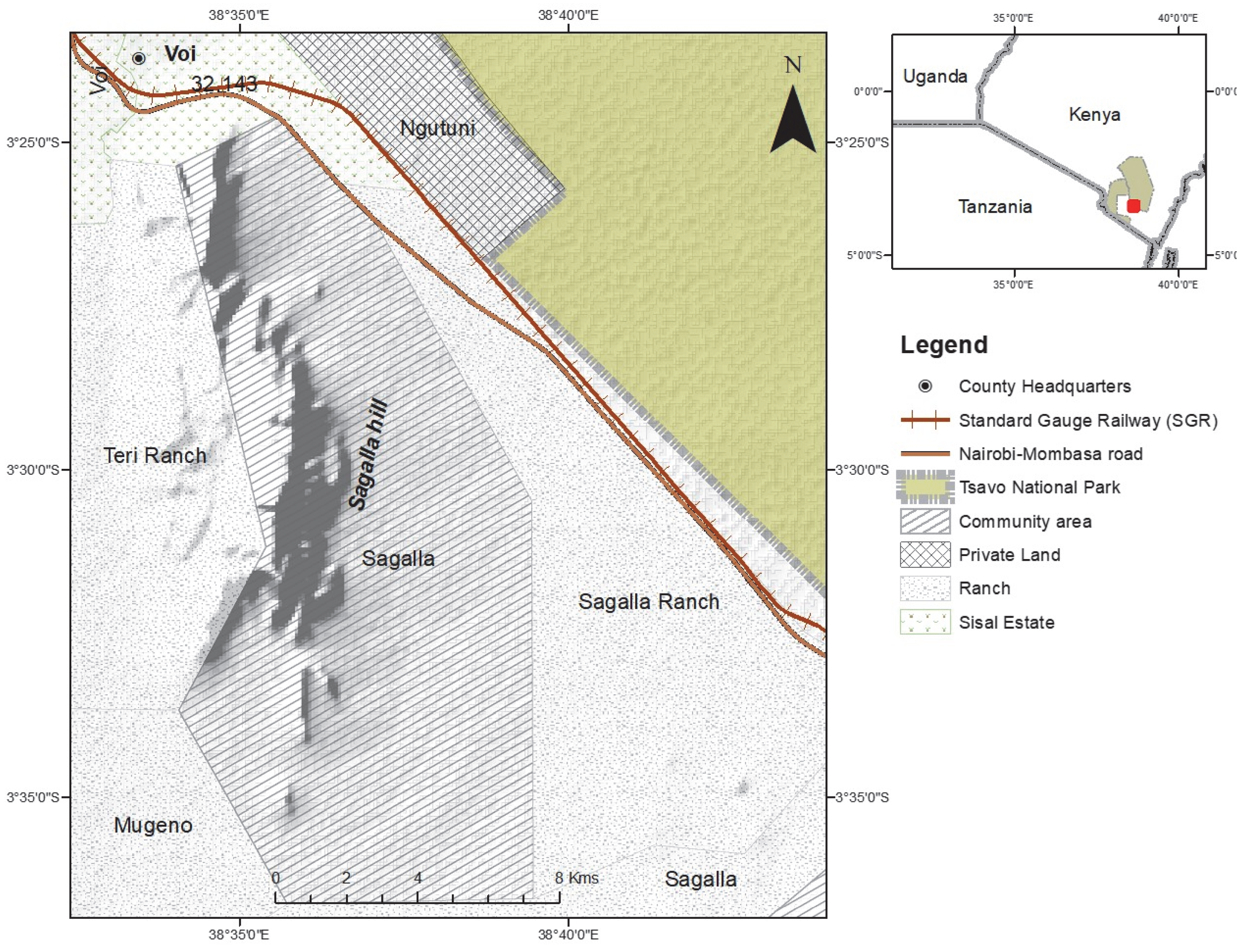
The study was conducted in the naturally vegetated area of Sagalla, south of the Sagalla hill (Figure 1). Agricultural farming is the main source of income for communities living at the bottom of the hill. The Sagalla area is located south of the Tsavo East National Park, situated 3 km close to the park boundary, and separated from the fence by the newly developed standard gauge railway (SGR) and the busy Nairobi-Mombasa tarmacked highway. To the east and south of Sagalla beyond the populated villages, there are large areas of natural vegetation, and partitioned ranches which still boast huge expanses of naturally vegetated land. To the west of Sagalla is the Sagalla hill where more farming is practiced at the top of the hill and is devoid of human-elephant conflict. Land to the south-west of Sagalla is partitioned as ranches but with mostly natural vegetation cover and hence wildlife presence. These ranches are left open with no fences to allow the free-flow movement in and out of the ranches. Elephants migrate north and south between the parks and hence pass through the Sagalla community area where we are presented with cases of human-elephant conflict. It is in this Sagalla community area that we have documented micro-movements of elephants from the Tsavo East and West National Park boundary fences into the community area and back, raid crops and destroy farm properties such as water tanks and houses within the period 2015 to January 2020.
2.2. Product Description and Pre-Processing Techniques
Sentinel 2A is a polar orbiting, multispectral, and high-resolution imaging mission. Sentinel 2A instrumentation comprises of 13 spectral channels, captures a swath width of 290 km allowing for large scale main category mapping, and bands at a spatial resolution of 10 m (4 visible and NIR bands), 20 m (6 Red-edge/SWIR bands), 60 m (3 atmospheric correction bands). Sentinel 2A data is available for free download from ESA Copernicus website [59]. Copernicus have also provided SNAP (Sentinel Application Platform) software from which to conduct spatial analysis on the Sentinel 2A imagery.
The downloaded product for Sentinel 2A satellite mission was product Level 1C (L1C) Copernicus Sentinel data 2017, retrieved from ASF DAAC on 26-01-2017, processed by ESA. This product’s description indicated that it had already been taken through several pre-processing stages namely; (i) telemetry analysis and decompression of the downloaded product at Level O, (ii) radiometric correction and geometric model refinement using the default 90 m SRTM DEM and global referencing images at Level 1A, (iii) resampling and conversion of pixel values to Top of Atmosphere (TOA) reflectance at Level 1B, and (iv) correction for gas and smile and water vapor retrieval, finally outputting Level 1C and cloud masks.
The radiometric correction performed on the L1C corrects for dark signal attributed to sun angle effects, pixel response non-uniformity, crosstalk, and identifies defective pixels that can be masked out ahead of processing. It also restores the high spatial resolution bands by noise removal and de-convolution. This pre-processing information is as provided for in the online Sentinel technical guide as captured in their website [60].
As illustrated in Figure 2, we introduced the downloaded L1C product into SNAP environment whereby the TOA reflectance passed through the Sen2Cor processor for terrain, cirrus and atmospheric to derive a sentinel L2A BOA product. We performed several alterations to the Sen2Cor configuration settings in L2A_GIPP.xml to facilitate cirrus removal and BRDF correction and defining the amount of cloud detection by setting the WV cirrus threshold to 0.25 < 0.34.
During the time of processing, sen2three product was not available to process 2017 sentinel 2A imagery. Sen2three toolkit replaces bad pixels (no data, saturated, defective, dark, cloud shadows, unclassified, medium and high probability clouds, thin cirrus and ice or snow) of an image with good ground pixels (vegetation, soil/rock, water, built surfaces) of recent or current earth observation imagery. There are a variety of algorithm options that can be determined in the configuration stages which include; (i) most recent- whereby bad pixels of the previous scene are replaced with good pixels of the most recent scene in the collection, and (ii) temp homogeneity- whereby previous scene pixels are replaced only if the sum of current scene pixels is higher than the best of the most current scene.
Failure to perform further image enhancements using this Sen2three toolkit to replace bad pixels, we masked out cloudy areas and shadows. The L2A output was resampled to 10 m spatial resolution to facilitate reprojection to UTM projected coordinate system. This output was then exported with the (.evf) extension to facilitate further processing in the ENVI environment. ENVI processing involved layer-stacking bands 2-8A,11 and 12, mosaicking, using color composites to visually pick out training regions, and supervised classification using maximum likelihood classification.
We developed comparisons between Landsat 8 and Sentinel 2A band resolutions to define suitable feature identification composite band combinations using bandwidth information as in Table 1 and Table 2. We compared the bandwidth positions of Sentinel 2A bands electromagnetic spectrum and cross-checked the best fit along the Landsat 8 spectrum. Sentinel 2 band 8A is specifically chosen for atmospheric applications instead of band 8 as is indicated in the Sentinel 2A user guides.
2.3. Supervised Classification
In ENVI environment, we applied false colour composite band combinations to define pixels or polygons to be used as training regions. The true colour rendition displays the red, blue, and green bands such that the output image is as close as possible to reality. Bands in the visible and NIR spectrum are used to detect photosynthetic vegetation while the SWIR contribute to separate individual contributions of non-photosynthetic and bare-soil structures. To distinguish vegetation features, a colour composite including the Near-IR band 8 is used. Green vegetation reflects Infrared light energy that is depicted on the image as the very red feature. Shades of red illustrate the different vegetation signatures on the landscape dependent on the leaf and canopy structure composition. Utilizing the Shortwave IR band 2000 nm to 2300 nm greatly and accurately improves the sub-pixel fractional covers of photosynthetic, non-photosynthetic and baresoil constituents’ estimation. Sentinel 2A provides a spectral coverage of 2100 nm to approximately 2380 nm in the Shortwave IR to carry out this level of feature distinction and extraction.
We generated Regions of Interest (ROI) to serve as the training areas upon which the cover types would be defined. The main training classes used as the benchmark for the classification define; grassland vegetation, forest vegetation, built-up areas, cultivated areas, water, wetland vegetation, shrubland, and bareland. To accommodate differences in canopy structures and standard dynamics, we branched out the training classes to create more ROIs. This was followed by conducting a measure of the separability between ROIs using the Compute ROI Separability tool option in ENVI between generated classes with close enough colour shades intensities while displaying the false colour composites. The ROI separability tool applies the Jeffries-Matusita distance and Transformed Divergence to output divergence metrics between defined classes and values it ranging from 0 to 2.0. A return of 2.0 means that the ROIs are completely separable and there is confidence in running them through the classifier. A return of metric values between 1.9 and 2.0 means that the ROIs have overall good separability and can be passed on to the classifier, but with potential of pixel misclassification if they are between 1.90 and 1.98. For values less than 1.9 it means the ROIs have fair separability, and the classes should either be merged to avoid misclassification [61], or they should be split further if having distinctly separable spectral signatures for classification, allowing for an option of recombining them post-classification. We used the n-dimensions (n-D) visualizer tool to further validate the uniqueness of these ROI pixels. The n-D visualizer generates a spectral scatter plot, where n represents the number of bands. For our application, the ROIs were plotted in a 10-axis plots, equivalent of the 10 bands used in the classification process. The coordinates of the ROI points in the n-D space consist of 10 spectral reflectance band values for each ROI pixel. Our direct import of the ROIs to the n-D visualizer was not based on the purest image pixels, hence it is possible some endmembers would miss in the resulting scatter plot. Endmembers are considered spectrally unique pure pixels that occur in an image scene and can be generated using a linear unmixing model.
ROI feature extraction was achieved by digitizing points and polygons using the ROI tool dialogue. The generated Image, Scroll and Zoom display windows are used to pan across the landscape. The Zoom display is used to digitize the training pixels, using the Image window to instantly pan onto that same area on Google Earth imaging platform in true color display. This step is crucial to affirm cover type characteristics and make an informed decision of the large-scale vegetation structure and land use characteristics. Several training sites are developed for generated classes, with the option of branching out and creating new classes that would adequately describe the complexity of the local vegetation pattern at the 10 m spatial scale, whose distinctive difference from training pixels of a similar class is determined using the separability tool and n-d visualizer. This refines class definitions to decrease ambiguity ahead of adopting the Maximum Likelihood Classification system for this classification.
2.4. Ground Truthing for Species Identification and Verification
We collected referencing data and measurements to observe the ground occurrence of the vegetation in the period from May 2017 to June 2018. This process was both expensive and consumed a lot of personnel time capacity taking extra caution accessing sampling points in densely forested areas as well as being on the look out to avoid any contact with wildlife. We involved local and professional botanists with deep knowledge of the local vegetation, as well as security personnel during these field expeditions. The ground truthing was essential in the interpretation of each cover type phenomena. Through comparison of randomly selected sampling points, it aided in the analysis of species contribution to the spectral information. This analysis obtained the quantitative estimates relevant to class distributions. A selected number of ground truthing points of known species locations, depicting high concentrations for the specific species were used in the validation of the supervised classification accuracy level.
Since the satellite data spatial resolution used was at 10 m, we determined that we would study the present vegetation species at 10 m radius from the sampling point’s geographical location. We used A GPS Garmin eTrex 20× to get to the sampling point locations set at 3 m accuracy ensuring at least 8 satellites were locked in before recording data. Some sites were densely forested so, aware of the risk of a weakened signal and potential for error, we maintained collecting data on the species in a 10 m radius from the central GPS point so long as the GPS locked in a minimum of three satellites [62].
We selected several sampling sites per classification class to determine species dominance. We then used this data to define the plant community based on quantifiable parameters. At each sampling site we collected species data based on percentage frequency and percentage cover. In some instances, we made computations of species density to supplement the spatial record of occurrences in places with a variety of tree species. Recorded field data comprised of:
- i.
- Frequency- the number of quadrats within which an individual species appears
- ii.
- Cover and Density- combined influence of the percentage of ground covered by a species determined by the size of canopy viewed form an aerial perspective, collected from the top (trees) down (shrubs), as well as a head count of the number of individual species occurring at one sampling point. Done for sampling plots with numerous numbers of tree and shrub species.
2.5. Species Dominance Characterization
This was achieved by determining the Importance Value Index (IV) of the vegetation specie composition within 10 m radius of the GPS sampling point. The IV is the measure of the dominance of a vegetation species in a sampling plot. IV is the measure of species diversity and richness, whereby the vegetation data is quantitatively analyzed for relative cover and relative frequency [63,64,65]. The data collected and used to determine this includes (see Table 3):
- Relative frequency- this is the percentage of points occupied by a specific vegetation specie as a function of all species present
- Relative cover/abundance/density- which is the number of individual vegetation species in an area as a percentage of the total individuals of all vegetation species
The equations used to calculate the IV for each cover type include [66]:
From the raw species’ cover observations per ground truth site , is the cover or abundance of each vegetation species type where is the individual species type. is the total number of sample ground- truthing sites for each classification class Cover was determined using:
where the cover of the species and is the sample plot identity, is the total cover area of a sample plot in this case documented as 1 to represent the complete 10 m radius from central GPS point location, while the estimated score count in percentage based on the Braun-Blanquet abundance/cover scale [67] shown in Table 4 for species in sample plot , as well as an informed estimate ‘by eye’ of top-down canopy cover and tree height position influence.
We followed this with computing for the relative cover
where all species occurring within each plot and is the relative cover in percentage of each individual species. The relative cover of an individual species across all ground truthing plots for each classification class was computed as
The relative frequency for each individual vegetation species within a classification class was determined using
where is the relative frequency of an individual species , is the total number of plots in which the individual species occurs, and is the total number of sample plots used to ground truth for a specific classification class .
The Relative Importance Value index (RIV) was determined further down the line from the Importance Value index (IV) which was the summative value out of 200% of the relative frequency and the relative cover as in
for all the vegetation species occurring in a specific classification class This result would equal to 200% for classification class, and would then be divided by 2 to give the RIV resultant value out of 100% to represent the dominance of an individual vegetation species in the associated classification class hence:
Using the RIV dominance values per classification class, we could now proceed to assigning names of classification classes based on the floristic association technique, where the scientific names of the most dominant vegetation species are used.
2.6. Naming Floristic Association Vegetation Classification Classes
We followed the nomenclature rules and guidelines for assigning of ecological community scientific names [34], to the vegetation classification classes for which we had sampled adequate ground truthing data. Association names require a maximum of five species which would be necessary for the classification classes with very diverse species types of considerably even dominance RIV values and varying total composition, for purposes of clarity. However, fewer species names are desirable in the final name. We assessed the top five RIV species for each classification category and determined how many species would be present in the name dependent on the spread of dominance value positions. We considered the species to be occurring in the same stratum hence the species labels were separated using , a hyphen with spaces. Therefore, the order of species in the assigned association level name would reflect decreasing dominance level. Where the complete species name was not known, we used the general term spp. as the species placeholder, for instance Indigofera spp. At the end of each association name, we added the general classification type such as ‘grassland’, ‘woodland’, or ‘shrubland’.
2.7. Introducing Elephant Tracking Data and Analysing the Relationship with Vegetation Communities
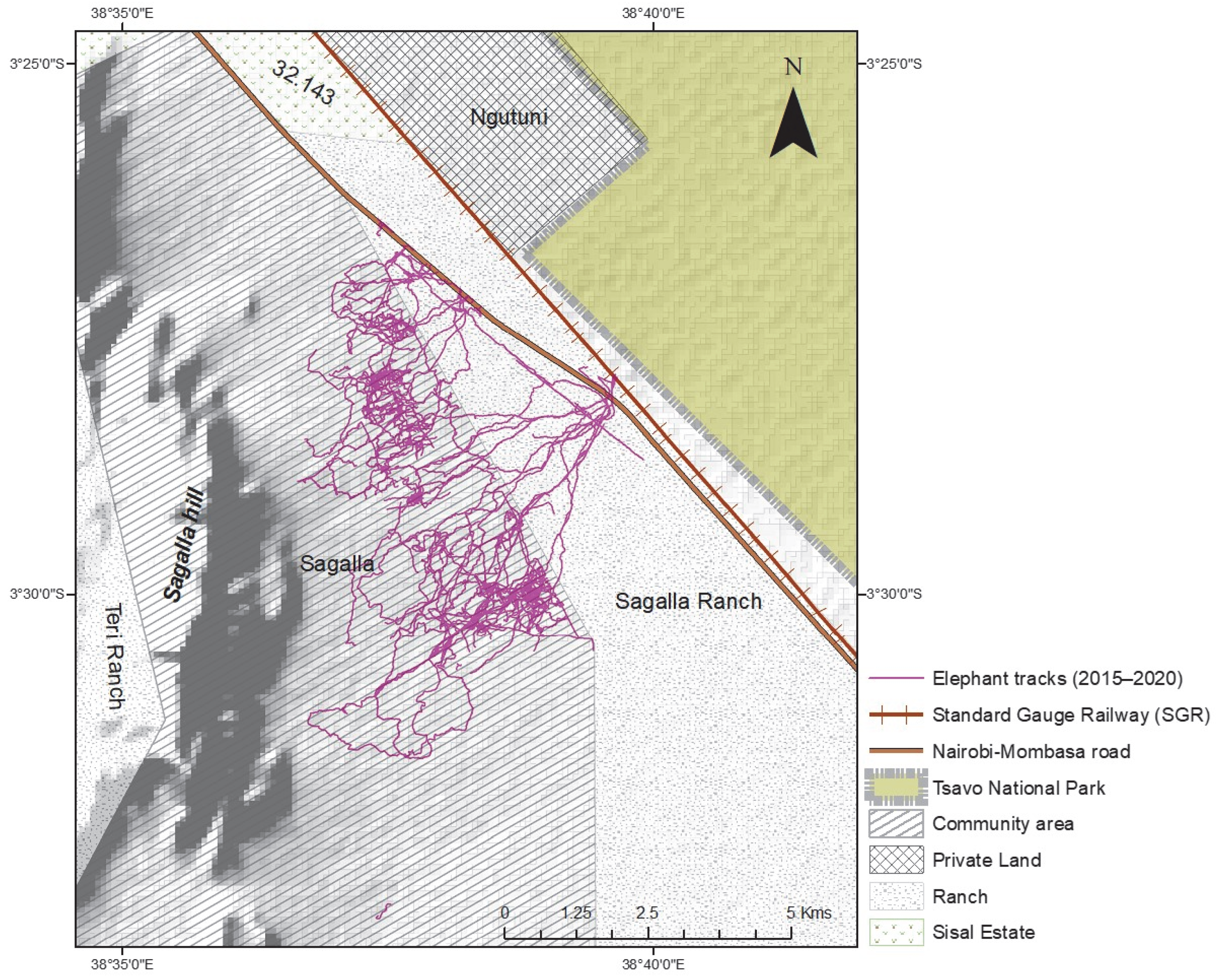
We incorporated the in person-collected elephant tracking data collected by our team at Save the Elephants over six years from 2015 to January 2020, a total of 268 tracks across this community area and ranch landscape (Figure 3). Each elephant movement track applied in this study was collected the day following an elephant raid or visit event using the mobile handheld Garmin etrex GPS on foot, from a starting point within the community area or park fence and following the elephant footprints (measured for accuracy purposes) up to where the field team either loses the track or meets a barrier like the park fence, or in extreme cases, came close to the elephants they were tracking. The tracks were recorded as points in GPS Exchange format (gpx). Each point of a typical gpx track contained; an identity label, latitude and longitude coordinates, a local time stamp, and elevation data. The total movement data recorded and used in this study was about 447 km, with the shortest track being about 200 m and the longest about 30 km, and the mean of all tracks being 1.7 km. The map shows the extent of the elephant tracks across the study area landscape. They traverse the area comprised of natural vegetation and into the farms. Farm areas are excluded from this study as we only assessed the influence of natural vegetation species as a motivation to their movement patterns and location.
We used the raw point movement data to extract the classification output raster values to each point. We then performed summary statistics on the extracted data to extract information on which movement points fell within each classification class, as well associated attribute information of the gender grouping of the elephants, as well as the minimum and maximum number of elephants recorded to have followed the associated track.
3. Results
3.1. Band Correlation and Selection for Training Regions of Interest (ROI)
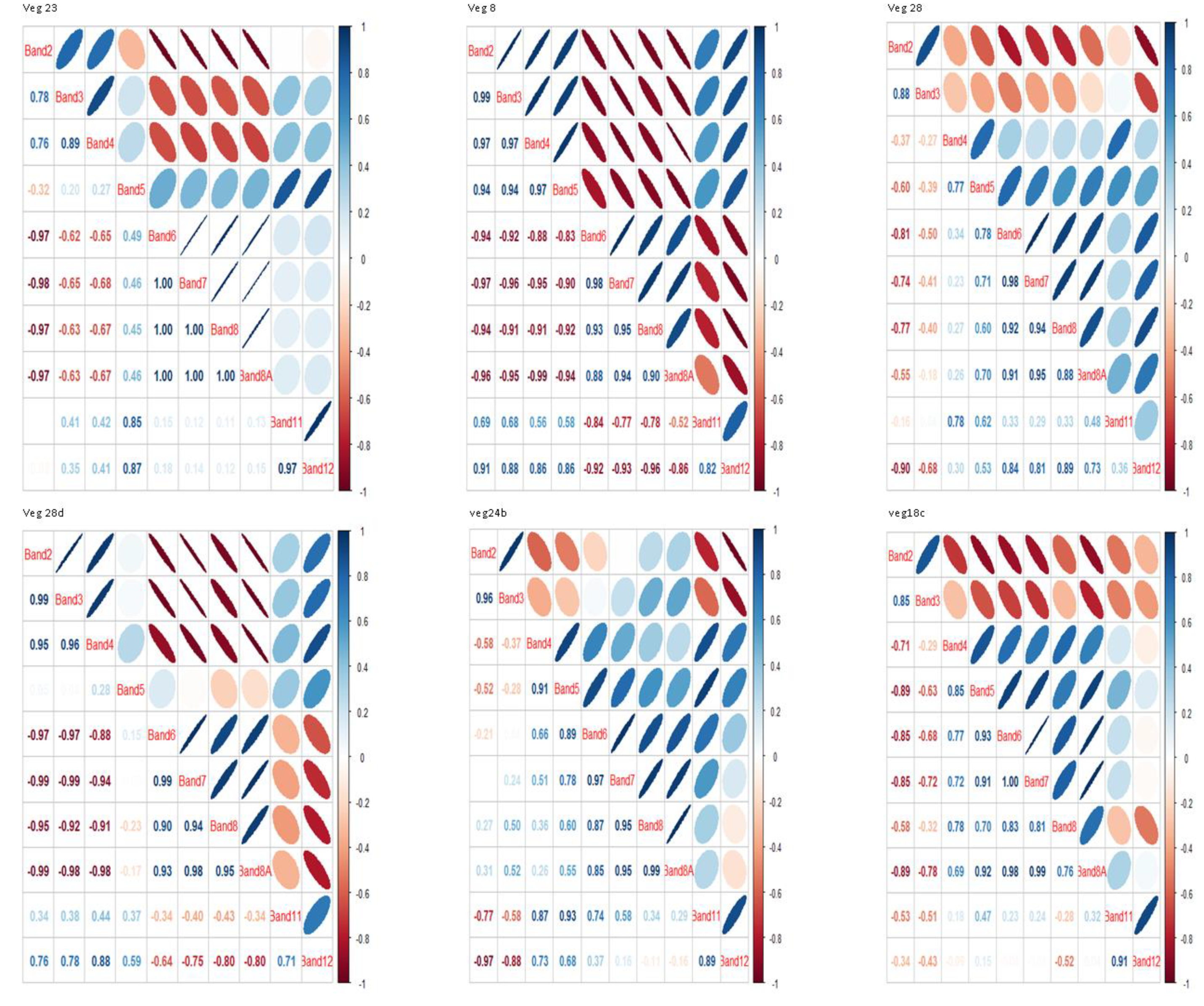
Correlation coefficients of the reflectance between band pairs for each of the ROI training pixels were computed to determine the degree of correlation (Figure 4).
Of the bands 6, 7 and 8 that showed very strong correlations, band 8 was considered to be of the greatest importance for inclusion in the color composite process to aid in identifying areas to assign to specific ROI classes since the NIR radiation aids in detecting vegetation densities in both densely and sparsely vegetated areas [68]. Since band 11 is lowly correlated to the rest of the bands in all the ROI classes except for veg24b, it is a suitable band to use for the color composite as it would add value that would further aid in the feature identification process for the vegetation ROIs. Band 8A and band 8 which consistently showed very strong correlation were applied interchangeably to help reinforce feature identification with the color composites. Bands 3 and 4 showed different strengths in correlation for different ROI selections; they were strongly positively correlated for veg28d, veg8 and veg23 ROI assigning and weakly negatively correlated for veg18c, veg24b and veg28. Bands 3 and 8 were very strongly negatively correlated for veg28d and veg8 and moderately negatively correlated for the other ROI classes. Interestingly, bands 4 and 8 showed similar trends of very strong negative correlations for the same veg28d and veg8, but unlike with band 3, they showed moderately positive correlations with the rest of the classes except veg23 where it showed moderate negative correlation.
From the standard deviation statistics for all ROI pixels chosen for the training classes shown in Figure 5, the spectral signatures at band 8 and band 11 are the most distinguishable across most classes. The standard deviation at band 3 show spectral signatures that are very close to each other, but clearly distinguishes between Veg24c and Fvg1c. Band 11 shows distinct differences in standard deviation values for all the ROI classes. Band 4 and band 8 have fairly good distinction between the ROI classes seeing from the spread of the standard deviation values.
The ROI separability tool used to ascertain the ROIs were spectrally separable enough to be assigned different classification classes output values ranging from 0.0 to 2.0 as a metric of separability between any two ROI classes as in Table A2, shows two classes Fvg1c and Veg29c returned good separability values with class Veg24c, but with the likelihood of some pixel misclassification between them and Veg24c. Veg 16 is the only class that returned a metric value of 2.0 indicating very good separability when paired with all the other classes. The rest of the pairs returned good separability value between 0.98 and 1.999, giving confidence that these ROI pixels were good enough to be passed on to the classifier to assign pixels falling within their spectral range to respective classes.
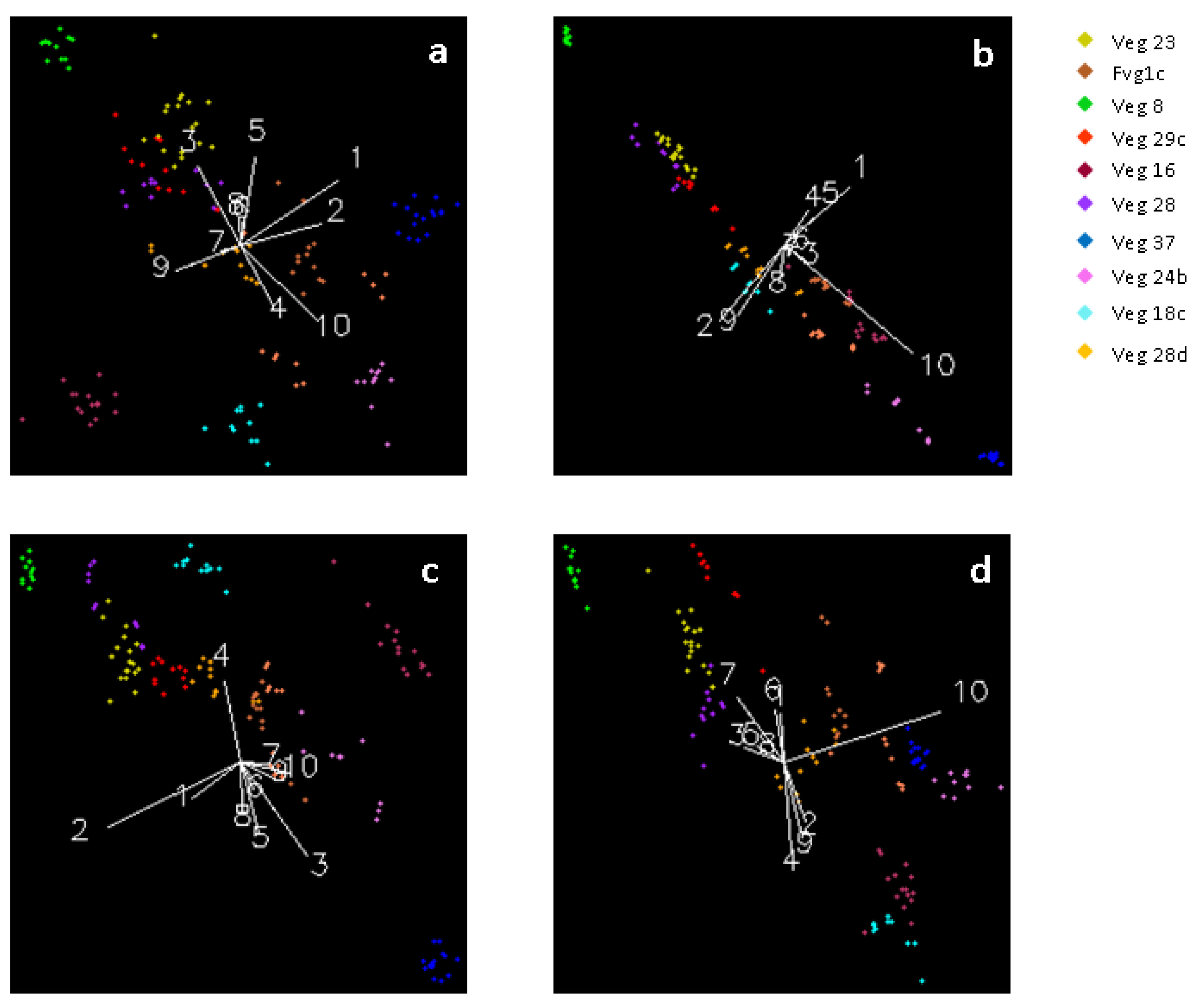
When viewed from these four dimensions on the n-d visualizer as in Figure 6, it is evident the ROI classes’ pixels cluster well. The Veg8 and Veg37 pixels are consistently clustered together, and thus it can be derived that these are spectrally unique pixels. The rest of the ROI pixels are clustered much closer to each other as in b, however, viewing them in other dimensions as in a, c and d on the 10-dimensional axis brings out clean clusters. Veg16, Veg18c and Veg24b pixels cluster purely as in views a, b and c, despite being located within the center region of the scatter plot, however, there is one Veg16 pixel that plots with Veg18c cluster as in view d. Veg28, Veg23 and Veg29c pixels cluster semi-purely as seen in views d and b, and evidently, there are is some overlap of Veg28 and Veg23 pixels plotting in each other’s spectral space as in views a and c. Fvg1c and Veg28d pixels consistently plot in common spectral space as in all views, with some pixel-overlap. As seen in view a, there is significant spread in the spectral space for the Fvg1c and Veg28d ROI pixels, hence they could potentially present mixed pixel spectral properties.
3.2. Post-Classification Accuracy Assessment
The confusion matrix returned results of an overall accuracy of 87.395%, and Kappa coefficient of 0.855. Most of the classes’ ground truthing ROIs used in the accuracy assessment were correctly classified into desired classes, while some had instances of the pixels being classified into other classes (Table A5 and Table A6). From the afore-mentioned tables, we find the classification results align with the spectral pixel-purity clustering (Figure 6) and ROI separability (Table A3) outputs. Veg8 and Veg16 ROIs that were found to be perfectly spectrally separable from both clustering in n-d visualizer analysis and the ROI spectral separability test, were also accurately classified with 100% ground-truthing pixels being correctly classified into their respective classes. We also find misclassification of pixels following a similar pattern from ROI selection to classification. This is evident in finding some ground-truthing pixels for Veg28 being classified as Veg23 as predicted by some of the ROI pixels plotting in the same space in the 10-dimensional visualizer. Some Fvg1c ground-truthing pixels were classified as Veg29c as could be expected from both the 10-dimensional clustering and ROI separability outputs, but at a low percentage of 8.3%. Similarly, the Veg29c classification of some pixels into Veg 24c follows the ROI spectral separability output that was 1.972186, a metric less than 1.98, but also at a low omission rate of 8.3% to this particular classification class.
3.3. Distribution of Species in Classification Classes from Ground Truthing Data
All classification classes had many vegetation species contributing to the community composition (Figure 7). More than half of these species in each community had a low dominance level based on their RIV value position of below 5. The RIV value positions of the most 2–3 dominant vegetation species are well above the interquartile range of all species forming the community. However, it is notable that the classification classes with minimal sampling plots below five had vegetation species with the highest RIV value, positioned as outliers well beyond the extreme upper quartile position. It is only in Bgv7 classification class that there are some species that fall in the lower extreme position of the interquartile range, based on information from three sample plots.
Classes with dominant species having RIV values falling between 10 and 25 indicate that these species are fairly equally balanced in presence, and hence have fairly equally matched contribution to the spectral uniqueness of the associated classification class. Classes with extreme outliers of RIV value over 25 indicate that these are the core contributor-species to the spectral signature uniqueness of the associated class.
As illustrated in Figure 8, classification classes bgv7 and veg 37 with less than five sampling plots and few vegetation species present; six and seven species, respectively, recorded their most dominant species as having very high RIV values of 48.2 and 44.5 respectively. This is unlike in the other classification classes that had more than five sampling plots and even more species of vegetation recorded as being present.
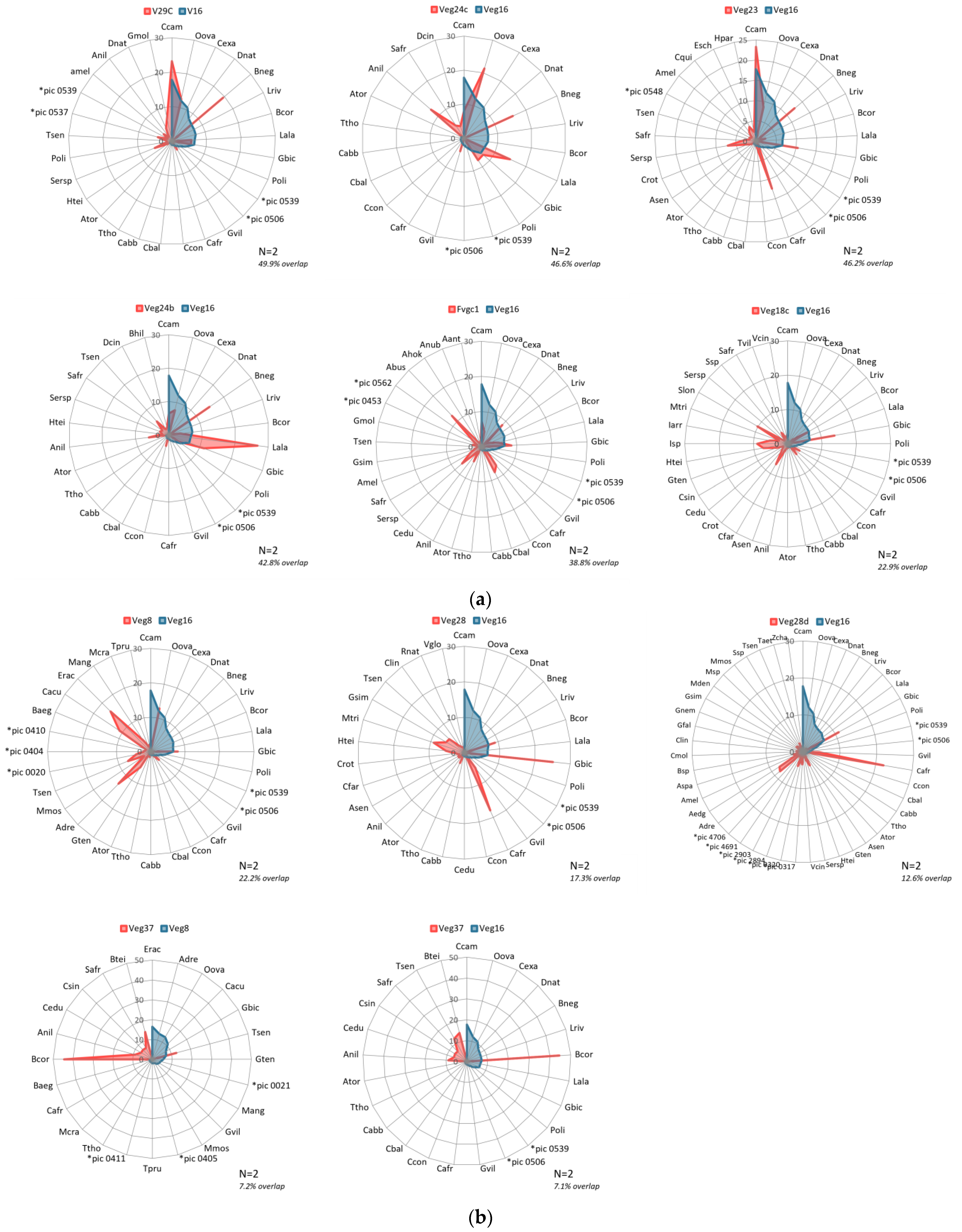
The ROI separability metrics output comparisons (Table A2) showed classification class Veg16 to be very well separable from all the other nine classes as it returned a value of 2. From vegetation species community information gathered from the sampling plots (Figure 9, Figure 10 and Figure 11), it is evident where there are overlaps in composition. Veg16 registers common vegetation species with Veg23, Veg24c, Veg24b and Fvg1c mostly (Figure 9a,b), but in very different quantities that when compounded with the other vegetation species that contribute to their distinct vegetation communities, it is enough to register distinctly different spectral signatures. In the afore-mentioned classes, the common vegetation species present across all five in varying dominance levels are the Commiphora campestris, Boswellia neglecta, Grewia bicolor and Ochna ovata. Interestingly, how the four vegetation species in these classes associate with each other in quantity and distribution, and with the addition of other differing vegetation species collectively determine that indeed these classes can be classified as different communities at such high resolutions, but in the lower resolutions, could have possibly been considered as one vegetation type. It is also interesting to note how the other classes register high quantities of other vegetation species and thus were classified as different vegetation classes.
Figure 10 illustration shows the three vegetation class pairings that returned values between 1.9 and 1.98, which are considered to have good separability and can be committed further to the classifier, but with the likelihood of resulting misclassification of pixels into the other classification class. From the vegetation species identified to be constituent in these classes, it is evident why the classes are considered to have good separability from the ROI separability results, but with caution. The comparison pairings between Veg24c and both Fvg1c and Veg29c shows considerable overlap in vegetation species compositions, but with very different dominance levels. There is also the contribution of other vegetation species unique to each of the classification classes.
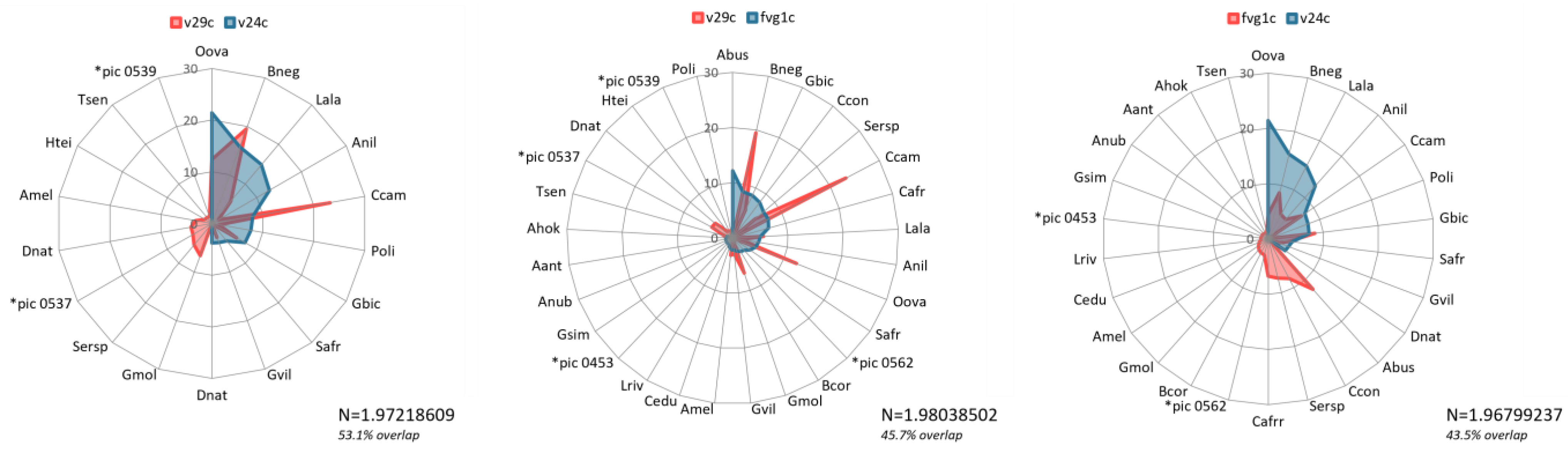
Figure 11a,b illustrations are for ROIs that qualified as having good separability and could be committed to the classifier. It is evident that they have common vegetation species occurring in the different pairings, but with considerable differences in dominance levels and other unique species present. These differences in associations potentially contribute to the more separable or distinguishable the vegetation classes and communities are. From these illustrations, we note that the ranking of ROI separability does not have a direct relationship to the order of ranking in constituent species’ overlap. We find vegetation community pairing between Veg24c and Veg28 (Figure 11b) with much lower ROI separability score to have much lower species’ overlap between them while a similar lower scoring pairing between Veg24b and Veg24 having a very high species’ overlap between the two classes. We also find a much higher ROI separability pairing result between classification classes Veg29C and Veg23 (Figure 11a) having a significantly higher species’ overlap between them. Despite these variations and the obviously significantly high species’ composition, we find that there are significant variations in dominant vegetation species and instances of unique species present within either of the vegetation communities, thus no two classification classes are the same.
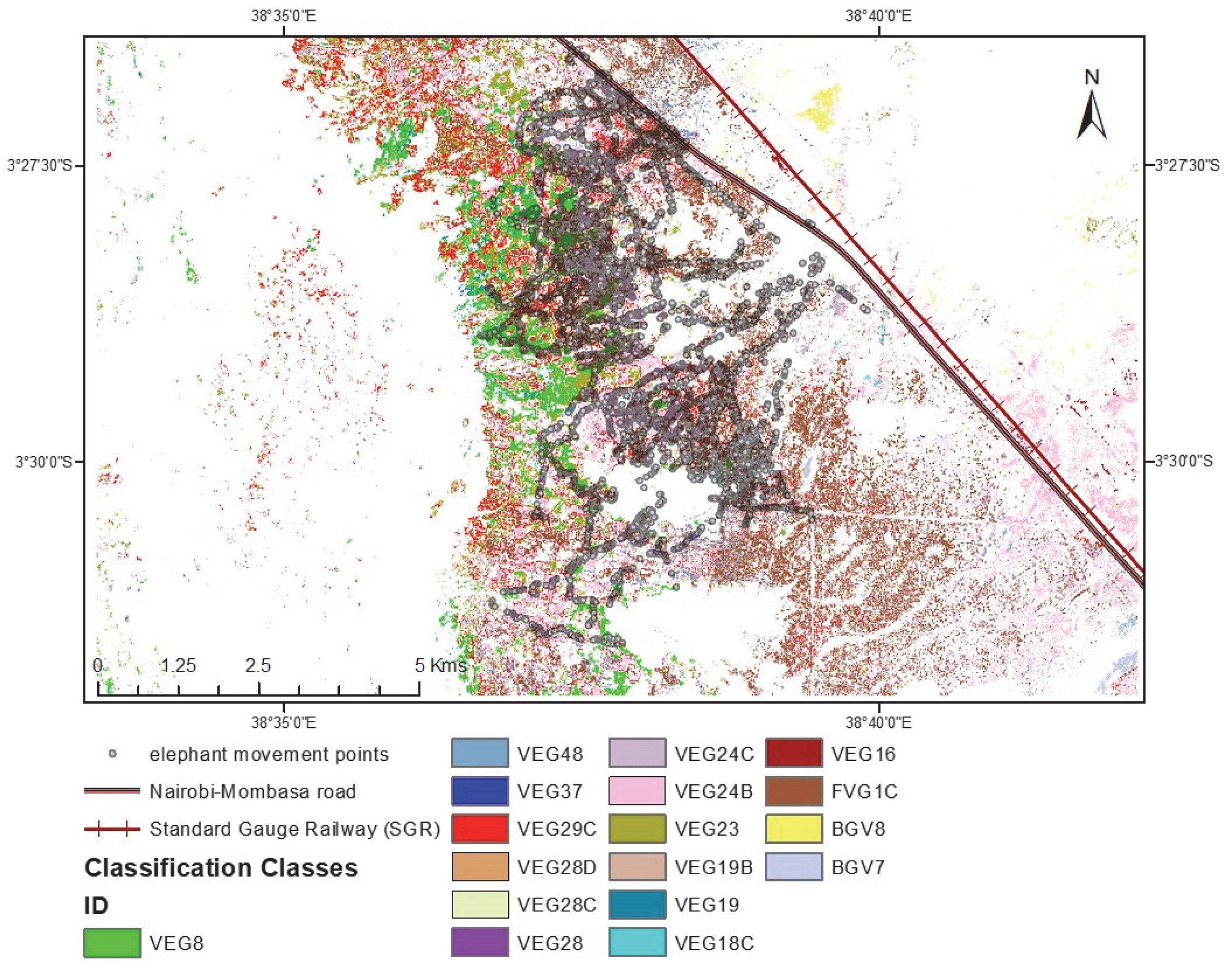
The classification output is as illustrated in Figure 12 below, overlaid with point elephant movement data. The associated statistical summary data was extracted from the point locations of the movement data resulted in the output illustrated in Table 5. The number of elephants recorded as + in Table 5 means that there were elephants present and whose track movement was recorded, but the field officers did not record how many. It is used as an elephant presence indicator in this case.
Figure 13 shows the resulting classification output whereby the vegetation classes are labelled based on the floristic-association with dominant species featuring in the label. The elephant tracking data have been redacted for this final map.
In Table 3, we find that the vegetation classified as Fvg1c is the region with highest elephant movement presence. Other key vegetation classes with elephant movement and presence recorded are the Veg24b, Veg24c, Veg29c, Veg23 and Veg8 in order of highest number of points captured when tracking using the mobile GPS, which recorded the maximum number of elephants in these regions as approximately 30, 20, 20, 20 and 15 respectively. Note that these huge herd elephant numbers were approximates, as in such cases very many footprints would be seen and recorded, in addition to witness accounts, and they would give a rounded off estimated of the elephant number count. These notable important vegetation class communities were also recorded as having been visited by families and herds with females and calves. Of the vegetation classes with lower presence point count such as Veg48 with 76 movement point and Bvg8 with 7 movement points, and Veg16 with 187 movement points, it is notable that these were instances with just elephant bull movements. Some elephant tracks did not have documented information on gender groupings.
3.4. Naming of the Vegetation Classification Classes Based on Floristic Associations
The resulting association names for the classification classes (Table 6) varied in number of species present in the name such that; 3 classification classes had just 2 species appear on the floristic-association name, and 7 classification classes had 3 species contribute, an indication that for these classes, the top two and three most dominant species, respectively, ranked quite high up relative to the rest of the species in that community to be significantly representative of the associated classification class. Four classes had 4 species on the association name, and three classes had all top five dominant species recorded on the association name. The classification classes that resulted in a four- or five- species name had species with RIV values with minimal spread, and hence it was necessary to include more species on the name list for clarity purposes. None of the classes had the same order of species names or composition, and hence these vegetation communities could be considered quite distinct.
4. Discussion
4.1. Image Processing and Analysis
A lot of the research and application within the scope of mapping vegetation cover using Sentinel 2A achieve high classification accuracies, however, literature shows that the interpretation and comparison of its application in this magnitude should be done with caution as the performance of the classifiers is subject to an array of factors including the training sample size [69,70], the number of classification classes [71], the terrain type [72], the preprocessing methods adopted [73], as well as the image interpretation adopted [74].
To commit to the training ROIs adopted in this research, we limited ourselves to a small number of training pixel samples of between 13 and 20 to run in the classifier shown in Figure 6. This can be subject to contradiction as different applications and scopes of landscapes under study will recommend using larger sample sizes of 50–100 pixels to improve the performance of supervised classifiers [75]. Further analysis of the spectral positioning of the training ROI pixels in the 10-Dimensional space (Figure 6) and the spectral separability (Figure 5) does in this case justify maintaining the classification training ROIs to the few samples to retain the uniqueness of the pixel properties of the collection. However, the size of the landscape, whether local or global, as well as the level of classification, whether community-level or species, are key determinants of the sampling level required to segregate close but different spectral signatures or combine spectrally similar pixels [76].
The spectral correlation was important to guide in the best band combinations for feature identification. Strongly correlated bands mean that the information therein is redundant and hence some of these bands can be excluded from the classification process. In our case, we used this information to determine the best bands for vegetation feature identification by helping accurately distinguish pixels when selecting ROIs. A positive correlation coefficient value means that as the value of one band increases, so does the other band value. A negative coefficient value in turn indicates that the two bands are inversely related. A correlation value of 0.8 and above means that the two bands are very strongly related, while a value of 0.5 means the bands are moderately related [32]. Bands 6, 7 and 8 were very strongly correlated hence we chose to use the NIR band 8. Green band 3 and Red band 4 were in some instances very strongly correlated and weakly in others (Figure 4), hence the inclusion of these bands in the band composites would be suitable for effective vegetation feature identification for some classification classes, and not the best for others. The standard deviation graph (Figure 5) shows the performance of band 11 in distinguishing between ROI pixels across all classes being better than band 3, thereby supporting the afore-mentioned findings. To further improve the vegetation feature identification for such classes, using the SWIR band 11 that is weakly correlated in almost all classes was sufficient. All bands were however used in the supervised classification process. Using the few interchangeably lowly correlated bands 11, 8, 4 and 3 relevant for vegetation feature extraction would probably improve the classifier performance by leaving out the highly correlated bands and thus eliminate redundancies. However, research has shown that using derived spectral indices as additional bands during classification would greatly improve the performance of the classifier [77,78,79], as earth observation data could be noisy, and the reflectance measured impacted by the satellite orbit position and angle. Determining the separability of training ROIs both spectrally and visually is a crucial step before committing the classifier. As illustrated in Figure 6 and Table A2, these two systems return results that aid in the determination of the uniqueness of pixels to be used as samples for accurate classification of vegetation. The clustering of ROI pixels in the n-dimensional visualizer is depictive of how similar or dissimilar the pre-selected spectral signatures are [62,80]. In addition to the ROI separability test results that return values ranging from 0.0 to 2.0; where a value of 2.0 means the ROI pixels are perfectly separated, while a return of more than 1.9 means they are well separated and hence classes are distinguishable, but with the caution that values less than 1.98 have the potential of miss-classification [61]. From the separability test output (Table A2), it is noted that the classification classes Veg24c, Fvg1c and Veg29c are separable, but since they return values less than or equal to 0.98, they have the potential of being mis-classified. On the 10-dimensional visualizer however, the pixels for these classes do not plot in the same space, hence the likelihood of them classifying the image distinctly enough.
4.2. Vegetation Communities’ Species Composition Analysis
Due to the time investment needed to conduct the field surveys at multiple sampling points for each vegetation classification, we limited our classification output to 17 classes for demonstrating outputs for this concept, out of the over 400 classes capturing the larger Tsavo landscape passed through the classifier and masked out the rest. Multiple randomly selected ground truthing plots were used to identify and quantify the concentrations of contributive vegetation species. Using the frequency and density values for each of the vegetation species in each plot, and further compounding the individual species presence across all plots for the associated classification class, we were able to compute the Relative Importance Value index (RIV) which determines the dominance position of each species within a class. The total number of plots used to determine the vegetation species compositions for each classification class varied, not by design, but what was achievable at the time. The number of plots used to sample for each class ranged from N = 12 to N = 2. We included the low plot sampling classes that had similarities between them in this classification but excluded those that had significant distinction to eliminate bias. However, it cannot be said for certain that those with plots samples of N = 3 and below in this output would have a significant shift in species’ RIV values from what is displayed. As for classes with plot samples of N = 5 and above, we have high confidence in the output of species’ compositions within the classification class communities from the consistencies across those plots.
Multiple approaches have been assessed to measure and map vegetation floristic compositions. Bazan et al. [81] found that measuring endemic and rare species using absence/presence data to determine the actual number of present species was efficient in assessing the quality of floristic landscape. However, Toumisto [82] intimates that such is related more to determining species diversity, and is not sufficient in mapping floristic associations as it does not take into account the influence of individual species’ abundances and proportions as we have in this study. Studies have also used the concept of Importance Value index to determine the dominant species and floristic compositions in respective study sites, similar to the approach in our research, with varying metrics in generating these IV indices such as the total basal metric of the tree community which is used by Chhetri and Shrestha [83] to compute the IV index and further determine ethe floristic composition.
It is evident from the boxplot in Figure 8 that multiple vegetation species contribute to vegetation communities in this region of study, many of which are in low concentrations. However, they are key contributors to the spectral signatures that make the classification classes separable in their own regard. The number of sample plots used to ground truth seem to be a significant factor in the range and distribution of species’ dominance values, as the classification classes Bgv7 and Veg37 (Figure 7) show. These two classes are on the high extreme of potential bias in what is classified as being the most dominant species with RIV values above 40%, much higher than the classification classes Veg16, Veg23, Veg28d and Fvg1c that have the most dominant species with RIV values between 10 and 25 (Figure 8). Of equal significance to determining the eventual dominance value of a vegetation species in a classification class is the number of species found present. The afore-mentioned classes that returned very high dominance values were also characteristic in having a lower count of vegetation species, and hence the only way to be certain that indeed these communities are thus constituted would have been to increase the number of ground-truthing sample sites, which would potentially have modified the present species’ list. The spectral signatures of most of the species indicated as having low dominance presence do contribute to the disparities in the communities that enables these classes to be spectrally different, in as much as there are the more dominant species that are graphed as outliers, and which would be useful in representing and naming the vegetation community.
The classification classes’ comparisons graphs show in greater detail the species contributing to each of the vegetation communities, and how they overlap in comparison (Figure 9, Figure 10 and Figure 11). Going back to the separability test results as well as the n-dimensional visualizer outputs, most of the community species’ comparisons overlap are consistent with what is expected from the classification (Table A3). It is expected that class pairs with ROI separability return of 2.0 should have minimal species overlap, while those of 1.98 and below have more overlap, and those between 1.98 and 1.99999999 have minimal species overlap. This is the case in most of these pairings. However, we find inconsistencies where despite the ROIs being perfectly separable with a value of 2.0 and purely clustered in the 10-dimensional visualizer, such as between Veg16 and Veg24b, there is a moderately high species overlap in the community compositions. Some results point to the n-dimensional visualizer giving a better depiction of the purity of pixels in instances where the ROI separability test returns values over 1.98. This is as evidenced in the species overlap between the Veg23/Veg29c, and Veg23/Veg28 pairs, which are very high and moderately high, respectively, consistent with the slight pixel overlap in the 10-dimensional space (Figure 6). However, it is notable that despite the high percentage species’ overlap (Table A2), the constituents forming these communities are variable enough to have made them be considered separable. Interestingly though, the dominant species in the Veg23 and Veg19c communities are quite similar, with them having the same two topmost dominant species Commiphora campestris and Boswellia neglecta; the most dominant (Commiphora campestris) has the same RIV values for both classification classes, and varying dominance of the Boswellia neglecta. Despite these two classification classes sharing common dominant species, there is significant variation in total species’ composition and dominance in the respective communities, which could have defined their separable nature as determined by the ROI spectral separability test. The composition of the class Veg28 is however very different to the other two in the leading dominant species, despite having some pixel-overlap in the 10-dimensional visualizer (Figure 6). From the above findings, we can determine that three factors; common vegetation types, varying dominance levels, and influence of unique vegetation types, are the reason why these classification classes should be maintained as distinctly different vegetation communities, and not generalized as one vegetation class.
4.3. Application of the Classification Outcome to Analyze Elephant Movement in Response to Vegetation Communities’ Species Compositions and Location
Classifying and mapping vegetation at such local scale into communities and naming them based on floristic associations provides information that is very important for ecological conservation applications, to understand the distribution, diversity and extent for in terrestrial wildlife species such as in this case the elephants [56,84]. Multiple factors influence the spatial distribution, movement patterns, and utilization of the home range of an elephant, including spatially variant anthropogenic, abiotic, biotic and physical factors [85], which we utilized in analyzing if indeed the location of select vegetation species in communities does impact elephant bull and family presence from the elephant micro-movement dataset in our study area.
Table 5 illustrates the presence and abundance occurrence of elephants in classification classes, which when tied to the acceptance rates of different vegetation types by different elephant groupings as fodder (Table A4), gives an idea of vegetation utilization within the different vegetation communities for the different elephant groups (Table 5). The elephant gender groupings illustrated here are: (i) bulls who either move as lone individuals or groups of several male elephants, and (ii) families which comprise of adult females and young calves of either gender. In few occasions especially when the adult bulls are in musth [86], they will be seen in the company of family groupings.
For this application, we were cautious to generalize the vegetation to genus level instead of species level as different species occur in different landscapes and available resources could not fully verify to the level of the specific species preferences local to our study area. Incredibly, we observed some trends that would be of interest as they show potential significance of vegetation species location to the movement of elephants; (i) all classification classes’ vegetation communities visited by elephant bulls only had a high or significant presence of Combretum, (ii) all visited by elephant families only had high or significant presence of Commiphora, (iii) classification classes visited by both bulls and families had vegetation accepted by either-or the elephant groupings namely: Commiphora for the family groupings, and Combretum and Cissus for the bulls. We also find that vegetation communities that had high numbers of elephants present at a time, that is more than five, consistently had high percentage of vegetation genus classified as acceptable fodder, while those with few elephants present at a time, that is five or less, had lower percentage of vegetation genus types regarded as acceptable fodder for the respective elephant grouping (Table 5). This analysis only considers fodder acceptance or no acceptance and does show the need for a clearer understanding and assessment of vegetation species communities’ locations as a measure of conserving the ecosystems that are key for the sustenance and survival of terrestrial wildlife species such as the elephant. Further information on the specific fodder vegetation species for elephants in similar study areas and verifiable quantifiable measurements would be needed to accurately classify preferable vegetation species based on acceptance metrics, which would then feed into the vegetation community map for elephant and vegetation management and conservation applications. Likewise, it would be valuable for future studies to include detailed foraging activity by elephants in each of these vegetation communities to better understand individual plant choices by elephants when variable forage are available.
Scientific knowledge of the vegetation ecology at species and community level for local applications is crucial for informed management of the key species for the survival of the wildlife species such as elephants used in this study. Location information of the key species as well as the vegetation communities utilized by elephants as key fodder would enable local authorities plan, advise, and engage local communities in efforts to conserve these vegetation communities against human invasion and destruction, if they cannot, by law, be sectioned out as protected areas.
4.4. Research Limitations and Future Works
Despite Sentinel 2A proving sufficient for classifying vegetation communities at species level at 10 m spatial resolution, the presence of clouds in imagery still make it a challenge achieving classification results of complete landscapes. However, new approaches have been developed to solve this issue by replacing bad or cloud and shadow pixels with good pixels from satellite scenes of a different moment in time when there were no clouds [87]. Original spectral information of all 10 bands was applied in the supervised classification in this study, which would have potentially improved the result if only uncorrelated bands as well as derived spectral indices would have been used as the input bands for classification [77,78,79].
This study took a lot of time especially conducting the ground truthing field studies. It is quite possible that there could have been modifications in the species compositions at study sites, arising from human influence such as logging as well as wildlife influences. There is also the potential for the GPS position for sample plots’ locations to have slight shift from the exact point owing to errors resulting from reduced satellites locking in in densely vegetated areas. This would require using higher accuracy survey equipment to verify and ensure positional accuracy during data collection [88].
More studies should be conducted to investigate the locally specific vegetation species that are utilized by elephants if the intended application is as in this study. This would ensure the local authorities are well informed to manage their local landscapes, which would mean quite a lot of time and work input in developing an accurate database for such applications.
5. Conclusions
The loss of biodiversity and species richness to utilization, transformation and degradation of natural vegetation by human influence especially in areas bordering protected areas can be detrimental to both wildlife species and humans. There is a crucial need to understand the locations and compositions of important vegetation species that are key fodder for wildlife, that would need protection to ensure availability as well as sustainable utilization of the resource. With this knowledge available, programs could be created to educate both the native communities, governments and interested conservation partners to manage sustainable use of the natural vegetation on a large scale, while concurrently putting measures in place to secure and redirect wildlife from destroying property such as crops. In this study, we proposed using Sentinel 2A for mapping vegetation communities at species level, based on their floristic associations. We tested the suitability of specific spectral bands to distinguish and help select the sample pixels to be used as training regions for image classification, being careful to assess the spectral uniqueness and potential success distinguishing quite similar but differentiable vegetation communities. Furthermore, we evaluated the applicability of the resulting vegetation communities’ information in assessing potential vegetation species’ and communities’ influences to elephant movement. We found that indeed Sentinel 2A imagery at 10 m spatial resolution is suitable for distinguishing vegetation species’ communities based on floristic associations, with the potential of improved outputs with the use of derived spectral indices. We also found that elephant movement is to a significant extent influenced by the geographical location of key species, as well as the community compositions and dominant species. Sentinel 2A multispectral imagery creates a suitable opportunity for application in mapping of vegetation at floristic association level at any location globally, and with the capacity of continuous monitoring that would greatly cover the knowledge gap of local vegetative influencers of wildlife movement, with the aim of conserving key species, as well as enhancing sustainable utilization, unique to specific locations. Understanding key movement drivers for wildlife like the elephant creates an opportunity to enforce informed conservation and management action. These could vary very much depending on location and the differences in vegetation communities across different landscapes, hence localized investigations should be done to inform local land owners and managers, and conservation enforcers. Further research should be undertaken in regard to zeroing in on accurate estimations on specific vegetation drivers to wildlife and elephant movement at this high resolution as what we have shown here is a clear indications on the correlation, however, improving our study with more data to explore statistical estimates would allow for stronger modelling for scaled conservation applications.
Author Contributions
Conceptualization, G.M. and L.K.; methodology, G.M.; software, G.M.; validation, G.M.; formal analysis, G.M.; investigation, G.M.; resources, G.M.; data curation, G.M.; writing—original draft preparation, G.M.; writing—review and editing, G.M., L.T. and L.K.; visualization, G.M.; supervision, L.K.; project administration, G.M.; funding acquisition, L.K; supervision, L.T. All authors have read and agreed to the published version of the manuscript.
Funding
This research received no external funding.
Data Availability Statement
The data presented in this study are available from the corresponding author, G.M., upon reasonable request.
Acknowledgments
We are deeply indebted to Save the Elephants and the Elephants and Bees Project, for creating an enabling environment to explore and channel our remote sensing interests and skills into this research. We give key mention and thanks to Anne Powys, an ethnobotanist with indigenous knowledge of local plants and their uses, who was the first person to plant the seed about doing a geospatial location-based study of specific vegetation species with respect to their utilization by elephants. This initial interaction with Anne and her passion for plants and wildlife interactions helped us conceptualize this study and ensured its successful completion. We express our appreciation to Festus Ihwagi at Save the Elephants for his invaluable consult in the early and intermediate stages of conceptualizing our methodology to ensure it was ecologically sound. His outlook of things from an ecological point of view was crucial to help us be objective and realistic in our goals and approach. We would also like to extend our thanks to Nashon Mwagharo, Oliver Tinga, and Francis Nyange, the local team that provided crucial security and transport support during the site field visits. Thanks to Muasa Mwololo and Esther Serem, for the invaluable knowledge on species naming and associated information they offered throughout the life of the project. Thanks to our core Tsavo field team who were involved in either elephant tracking or ground truthing data collection during the extended tenure of this project; namely Hezrone Nzumu, Emmanuel Mwambingu, Rohan Vince, Georgia Troup, Kennedy Leneuyia, Nashon Mwagharo and Marvin.
Conflicts of Interest
The authors declare no conflict of interest.
Appendix A

Table A1.
List of abbreviated vegetation species names.
| Abbreviation | Description |
|---|---|
| Abus | Acacia bussei |
| Adre | Acacia drepanolobium |
| Aedg | Acacia edgeworthii |
| Ahok | Acacia hokii |
| Amel | Acacia mellifera |
| Anil | Acacia nilotica |
| Anub | Acacia nubica |
| Asen | Acacia senegal |
| Ator | Acacia tortillis |
| Aant | Albizia anthelmintica |
| Aspsp | Asparagus |
| Baeg | Balanites aegyptica |
| Bhil | Blepharis hildebrandtii |
| Bsp | Blepharis sp. |
| Bcor | Boscia coriacea |
| Bneg | Boswellia neglecta |
| Btei | Bourreria teitensis |
| Cfar | Cadaba farinosa |
| Cabb | Cassia abbreviata |
| Cqui | Cissus quinquangularis |
| Crot | Cissus rotindufolia |
| Cacu | Combretum aculeatum |
| Cacu | Combretum aculeatum |
| Cexa | Combretum exalatum |
| Cmol | Combretum molle |
| Cafr | Commiphora africana |
| Cbal | Commiphora baluensis |
| Ccam | Commiphora campestris |
| Ccon | Commiphora confusa |
| Cedu | Commiphora edulis |
| Clin | Commiphora lindensis |
| Csin | Cordia sinensis |
| Dnat | Dichrostachys cinerea |
| Dnat | Diospyros natalensis |
| Ebus | Euphobia bussei |
| Erac | Euclea racemosa |
| Erev | Eclobium revolution |
| Esch | Euphobia scheffleri |
| Gbic | Grewia bicolor |
| Gfal | Grewia fallax |
| Gmol | Grewia mollis |
| Gnem | Grewia nemotopus |
| Gsim | Grewia similis |
| Gten | Grewia tenax |
| Gvil | Grewia villosa |
| Htei | Hilsenbergia teitensis |
| Hpar | Hymenodictyon parvifolium |
| Iarr | Indigofera arrecta |
| Imom | Ipoemia mombasana |
| Isp | Indigofera sp. |
| Lala | Lannea alata |
| Lriv | Lannea rivae |
| Mang | Maerua angolensis |
| Mcra | Maerua crassifolia |
| Mden | Maerua denhardtiorum |
| Msp | Maerua sp. |
| Mtri | Maerua triphylla |
| Mmos | Maytenus mossambicensis |
| Mvol | Melia volkensii |
| Oova | Ochna ovata |
| Poli | Premna oligrotirica |
| Rnat | Rhus natalensis |
| San | Sansevaria sp. |
| Slon | Senna longiracemosa |
| Sersp | Sericocomopsis |
| Ssp | Solanum sp. |
| Safr | Sterculia Africana |
| Tsen | Tennantia senni |
| Tvil | Tephrosia villosa |
| Tpru | Terminalia prunoides |
| Ttho | Thylachium thomacii |
| Taet | Tinnea aethiopica |
| Vglo | Vepris glomerata |
| Vcin | Vernonia cinerascens |
| Zcha | Zanthoxylum chalybeum |
Table A2.
A sample ranking of pairwise spectral ROI separability metrics for the 10 classification classes’ ROI pixels analyzed in this paper, from the lowest (in yellow) to the highest value (in green).
Table A2.
A sample ranking of pairwise spectral ROI separability metrics for the 10 classification classes’ ROI pixels analyzed in this paper, from the lowest (in yellow) to the highest value (in green).
| ROI Pairs | Separability Value | ROI Pairs | Separability Value | |||
|---|---|---|---|---|---|---|
| Fvg 1c and Veg 24c | 1.96799237 | Veg 8 and Veg 24c | 1.99999329 | Good separability with potential for misclassification | ||
| Veg 29c and Veg 24c | 1.97218609 | Veg 23 and Fvg 1c | 1.99999520 | |||
| Veg 29c and Fvg 1c | 1.98038502 | Veg 28 and Fvg 1c | 1.99999705 | |||
| Veg 28 and Veg 24c | 1.98476206 | Veg 8 and Veg 28d | 1.99999785 | |||
| Veg 29c and Veg 28d | 1.98476206 | Veg 23 and Veg 18c | 1.99999955 | Overall good separability | ||
| Veg 24b and Veg 24c | 1.99114939 | Veg 23 and Veg 28d | 1.99999984 | |||
| Veg 28d and Veg 24c | 1.99444385 | Veg 29c and Veg 8 | 1.99999986 | |||
| Veg 24b and Fvg 1c | 1.99461415 | Veg 23 and Veg 28 | 1.99999995 | |||
| Veg 29c and Veg 24b | 1.99682619 | Veg 8 and Fvg 1c | 1.99999999 | Very good separability | ||
| Veg 28 and Veg 8 | 1.99758124 | Veg 23 and Veg 24b | 2.00000000 | |||
| Veg 28d and Fvg 1c | 1.99777741 | Veg 24b and Veg 8 | 2.00000000 | |||
| Veg 29c and Veg 28 | 1.99839551 | Veg 23 and Veg 8 | 2.00000000 | |||
| Veg 28 and Veg 18c | 1.99919880 | Veg 24b and Veg 16 | 2.00000000 | |||
| Veg 24b and Veg 28 | 1.99964629 | Veg 18c and Veg 16 | 2.00000000 | |||
| Veg 28 and Veg 28d | 1.99985527 | Veg 28d and Veg 16 | 2.00000000 | |||
| Veg 18c and Fvg 1c | 1.99988690 | Veg 8 and Veg 16 | 2.00000000 | |||
| Veg 18c and Veg 24c | 1.99995738 | Veg 28 and Veg 16 | 2.00000000 | |||
| Veg 24b and Veg 18c | 1.99996309 | Veg 23 and Veg 16 | 2.00000000 | |||
| Veg 24b and Veg 28d | 1.99996485 | Veg 16 and Fvg 1c | 2.00000000 | |||
| Veg 23 and Veg 24c | 1.99996756 | Veg 29c and Veg 16 | 2.00000000 | |||
| Veg 28d and Veg 18c | 1.99997545 | Veg 16 and Veg 24c | 2.00000000 | |||
| Veg 8 and Veg 18c | 1.99998163 | Veg 16 and Veg 37 | 2.00000000 | |||
| Veg 29c and Veg 23 | 1.99998505 | Veg 8 and Veg 37 | 2.00000000 | |||
| Veg 29c and Veg 18c | 1.99999146 | Veg 23 and Veg 24c | 2.00000000 | |||
Table A3.
Percentage overlap of vegetation species present in classification classes paired for comparison. The colour scheme ranges from red with the highest species overlap to green with the lowest species overlap between any two vegetation communities.
Table A3.
Percentage overlap of vegetation species present in classification classes paired for comparison. The colour scheme ranges from red with the highest species overlap to green with the lowest species overlap between any two vegetation communities.
| ROI Pair Comparisons | ROI Separability Value | % Species Overlap | |||
|---|---|---|---|---|---|
| Veg 29c and Veg 16 | 2.00000000 | 49.96168678 | High | ||
| Veg 16 and Veg 24c | 2.00000000 | 46.55628785 | |||
| Veg 23 and Veg 16 | 2.00000000 | 46.15313425 | |||
| Veg 23 and Veg 24b | 2.00000000 | 45.3988607 | |||
| Veg 24b and Veg 16 | 2.00000000 | 42.83750912 | |||
| Veg 23 and Veg 24c | 2.00000000 | 40.88175714 | Low | ||
| Veg 16 and Fvg 1c | 2.00000000 | 38.78785074 | |||
| Veg 18c and Veg 16 | 2.00000000 | 22.99491533 | |||
| Veg 8 and Veg 16 | 2.00000000 | 22.23930848 | |||
| Veg 28 and Veg 16 | 2.00000000 | 17.28140071 | |||
| Veg 28d and Veg 16 | 2.00000000 | 12.59202352 | |||
| Veg 8 and Veg 37 | 2.00000000 | 7.190032803 | |||
| Veg 16 and Veg 37 | 2.00000000 | 7.107762041 | |||
| Veg 23 and Veg 28 | 1.99999995 | 33.83969365 | |||
| Veg 29c and Veg 23 | 1.99998505 | 59.16848829 | |||
| Veg 24b and Veg 18c | 1.99996309 | 27.88073058 | |||
| Veg 18c and Fvg 1c | 1.99988690 | 30.99680566 | |||
| Veg 28 and Veg 28d | 1.99985527 | 42.89996541 | |||
| Veg 24b and Veg 28 | 1.99964629 | 24.13941871 | |||
| Veg 28 and Veg 18c | 1.99919880 | 39.05253389 | |||
| Veg 29c and Veg 28 | 1.99839551 | 12.96072268 | |||
| Veg 28d and Fvg 1c | 1.99777741 | 22.90751023 | |||
| Veg 28 and Veg 8 | 1.99758124 | 20.21637096 | |||
| Veg 29c and Veg 24b | 1.99682619 | 47.44995034 | |||
| Veg 24b and Fvg 1c | 1.99461415 | 49.01213194 | |||
| Veg 28d and Veg 24c | 1.99444385 | 12.28768413 | |||
| Veg 24b and Veg 24c | 1.99114939 | 63.03686084 | |||
| Veg 29c and Veg 28d | 1.98476206 | 14.62957239 | |||
| Veg 28 and Veg 24c | 1.98476206 | 13.40523024 | |||
| Veg 29c and Fvg 1c | 1.98038502 | 45.70831551 | |||
| Veg 29c and Veg 24c | 1.97218609 | 53.12770883 | |||
| Fvg 1c and Veg 24c | 1.96799237 | 43.48403614 | |||
Appendix B
Table A4.
Vegetation utilized as fodder by African savanna elephants and their acceptance rates based on research done in South Africa by Greyling [38]. We use this information to determine the utilization rates by different elephant groupings in the vegetation communities as in Table 5.
| Acceptance Rates | ||||
|---|---|---|---|---|
| Bulls | Vegetation Types (Genus) | Family | ||
 | Acacia | | ||
 | Albizia | | | High |
| Combretum |  |  | Moderate |
| Cissus | | | Low |
| | Commiphora | | | No acceptance |
| Dichrostachys | | ||
| Euclea | | ||
| Grewia | | ||
| Lannea | | ||
| Maerua | | ||
| Terminalia | | ||
Appendix C
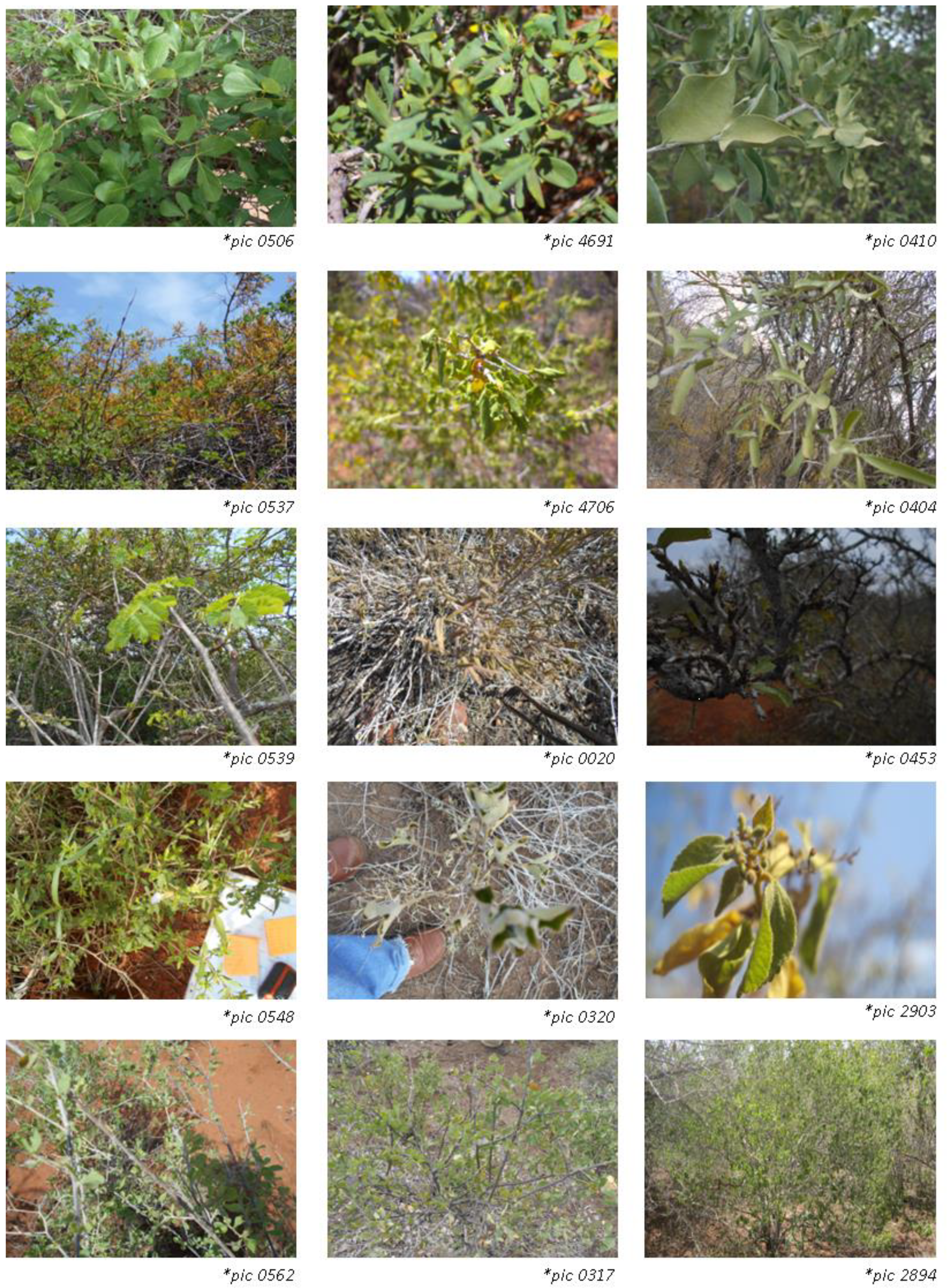
Figure A1.
Unidentified/unverified vegetation species by the end of this study.

Appendix D
Table A5.
Confusion matrix accuracy assessment output showing how the ground truthing ROIs were assigned by the classifier.
Table A5.
Confusion matrix accuracy assessment output showing how the ground truthing ROIs were assigned by the classifier.
| Ground Truthing (Percent) | |||||||||||
|---|---|---|---|---|---|---|---|---|---|---|---|
| gtveg8 | gtveg16 | gtveg23 | gtveg28d | gtfvg1c | gtveg24b | gtveg24c | gtveg29c | gtveg18c | gtveg28 | Total | |
| unclassified | 0 | 0 | 0 | 0 | 0 | 0 | 0 | 0 | 0 | 0 | 0 |
| VEG8 | 100 | 0 | 6.25 | 0 | 0 | 0 | 0 | 0 | 0 | 16.67 | 17.65 |
| VEG16 | 0 | 100 | 0 | 0 | 0 | 0 | 0 | 0 | 0 | 0 | 21.01 |
| VEG23 | 0 | 0 | 81.25 | 0 | 0 | 0 | 0 | 0 | 0 | 16.67 | 11.76 |
| VEG28D | 0 | 0 | 0 | 69.23 | 8.33 | 0 | 0 | 0 | 0 | 0 | 8.4 |
| FVG1C | 0 | 0 | 0 | 0 | 83.33 | 22.22 | 0 | 0 | 0 | 0 | 10.08 |
| VEG24B | 0 | 0 | 0 | 0 | 0 | 77.78 | 0 | 0 | 0 | 0 | 5.88 |
| VEG24C | 0 | 0 | 0 | 0 | 0 | 0 | 100 | 8.33 | 25 | 0 | 4.2 |
| VEG29C | 0 | 0 | 12.5 | 30.77 | 8.33 | 0 | 0 | 91.67 | 0 | 0 | 15.13 |
| VEG18C | 0 | 0 | 0 | 0 | 0 | 0 | 0 | 0 | 75 | 0 | 2.52 |
| VEG28 | 0 | 0 | 0 | 0 | 0 | 0 | 0 | 0 | 0 | 66.67 | 3.36 |
| Total | 100 | 100 | 100 | 100 | 100 | 100 | 100 | 100 | 100 | 100 | 100 |
Table A6.
The producer and user accuracies from the classifier performance as well as the percentage of ground truthing ROIs that were either omitted from or committed to the eventual expected class.
Table A6.
The producer and user accuracies from the classifier performance as well as the percentage of ground truthing ROIs that were either omitted from or committed to the eventual expected class.
| Commission | Omission | Producer Accuracy | User Accuracy | |
|---|---|---|---|---|
| Class | (Percent) | (Percent) | (Percent) | (Percent) |
| VEG8 | 9.52 | 0 | 100 | 90.48 |
| VEG16 | 0 | 0 | 100 | 100 |
| VEG23 | 7.14 | 18.75 | 81.25 | 92.86 |
| VEG28D | 10 | 30.77 | 69.23 | 90 |
| FVG1C | 16.67 | 16.67 | 83.33 | 83.33 |
| VEG24B | 0 | 22.22 | 77.78 | 100 |
| VEG24C | 40 | 0 | 100 | 60 |
| VEG29C | 38.89 | 8.33 | 91.67 | 61.11 |
| VEG18C | 0 | 25 | 75 | 100 |
| VEG28 | 0 | 33.33 | 66.67 | 100 |
References
- Charles-Dominique, T.; Davies, T.J.; Hempson, G.P.; Bezeng, B.S.; Daru, B.H.; Kabongo, R.M.; Olivier, M.; Muasya, A.M.; van der Bank, M.; William, J.M. Spiny Plants, Mammal Browsers, and the Origin of African Savannas. Proc. Natl. Acad. Sci. USA 2016, 113, E5572–E5579. [Google Scholar] [CrossRef] [PubMed] [Green Version]
- De Boer, W.F.; van Langevelde, F.; Prins, H.H.T.; de Ruiter, P.C.; Blanc, J.; Vis, M.J.P.; Gaston, K.J.; Hamilton, I.D. Understanding Spatial Differences in African Elephant Densities and Occurrence, a Continent-Wide Analysis. Biol. Conserv. 2013, 159, 468–476. [Google Scholar] [CrossRef]
- Blanc, J.J.; IUCN/SSC African Elephant Specialist Group; IUCN-The World Conservation Union. African Elephant Status Report 2016: An Update from the African Elephant Database; IUCN: Gland, Switzerland; IUCN: Cambridge, UK, 2003; ISBN 978-2-8317-1813-2. [Google Scholar]
- Calabrese, A.; Calabrese, J.M.; Songer, M.; Wegmann, M.; Hedges, S.; Rose, R.; Leimgruber, P. Conservation Status of Asian Elephants: The Influence of Habitat and Governance. Biodivers. Conserv. 2017, 26, 2067–2081. [Google Scholar] [CrossRef]
- Shaffer, L.J.; Khadka, K.K.; Van Den Hoek, J.; Naithani, K.J. Human-Elephant Conflict: A Review of Current Management Strategies and Future Directions. Front. Ecol. Evol. 2019, 6, 235. [Google Scholar] [CrossRef] [Green Version]
- Liu, P.; Wen, H.; Lin, L.; Liu, J.; Zhang, L. Habitat Evaluation for Asian Elephants (Elephas Maximus) in Lincang: Conservation Planning for an Extremely Small Population of Elephants in China. Biol. Conserv. 2016, 198, 113–121. [Google Scholar] [CrossRef]
- Mcdonald, R.I.; Forman, R.T.T.; Kareiva, P.; Neugarten, R.; Salzer, D.; Fisher, J. Urban Effects, Distance, and Protected Areas in an Urbanizing World. Landsc. Urban Plan. 2009, 93, 63–75. [Google Scholar] [CrossRef]
- White, P.C.L.; Ward, A.I. Interdisciplinary Approaches for the Management of Existing and Emerging Human–Wildlife Conflicts. Wildl. Res. 2010, 37, 623–629. [Google Scholar] [CrossRef]
- Newmark, W.D. Isolation of African Protected Areas. Front. Ecol. Environ. 2008, 6, 321–328. [Google Scholar] [CrossRef]
- Leimgruber, P.; Senior, B.; Aung, M.; Songer, M.A.; Mueller, T.; Wemmer, C.; Ballou, J.D. Modeling Population Viability of Captive Elephants in Myanmar (Burma): Implications for Wild Populations. Anim. Conserv. 2008, 11, 198–205. [Google Scholar] [CrossRef]
- Mariki, S.B.; Svarstad, H.; Benjaminsen, T.A. Elephants over the Cliff: Explaining Wildlife Killings in Tanzania. Land Use Policy 2015, 44, 19–30. [Google Scholar] [CrossRef]
- Tiller, L.N.; Humle, T.; Amin, R.; Deere, N.J.; Lago, B.O.; Leader-Williams, N.; Sinoni, F.K.; Sitati, N.; Walpole, M.; Smith, R.J. Changing Seasonal, Temporal and Spatial Crop-Raiding Trends over 15 Years in a Human-Elephant Conflict Hotspot. Biol. Conserv. 2021, 254, 108941. [Google Scholar] [CrossRef]
- Gubbi, S. Patterns and Correlates of Human–Elephant Conflict around a South Indian Reserve. Biol. Conserv. 2012, 148, 88–95. [Google Scholar] [CrossRef]
- Osborn, F.V. Seasonal Variation of Feeding Patterns and Food Selection by Crop-Raiding Elephants in Zimbabwe. Afr. J. Ecol. 2004, 42, 322–327. [Google Scholar] [CrossRef]
- Chiyo, P.I.; Cochrane, E.P.; Naughton, L.; Basuta, G.I. Temporal Patterns of Crop Raiding by Elephants: A Response to Changes in Forage Quality or Crop Availability? Afr. J. Ecol. 2005, 43, 48–55. [Google Scholar] [CrossRef]
- Branco, P.S.; Merkle, J.A.; Pringle, R.M.; Pansu, J.; Potter, A.B.; Reynolds, A.; Stalmans, M.; Long, R.A. Determinants of Elephant Foraging Behaviour in a Coupled Human-Natural System: Is Brown the New Green? J. Anim. Ecol. 2019, 88, 780–792. [Google Scholar] [CrossRef] [PubMed]
- Ngene, S.; Oduor, P. The Costs of Living with Elephants in the Areas Adjacent to Marsabit National Park and Reserve. Pachyderm 2009, 2009, 77–87. [Google Scholar]
- Sitienei, A.J.; Jiwen, G.; Ngene, S.M. Assessing the Cost of Living with Elephants (Loxodonta Africana) in Areas Adjacent to Meru National Park, Kenya. Eur. J. Wildl. Res. 2014, 60, 323–330. [Google Scholar] [CrossRef]
- Fernando, P.; Pastorini, J. Range-Wide Status of Asian Elephants. Gajah 2011, 15–20. [Google Scholar]
- Santiapillai, C.; Wijeyamohan, S.; Bandara, G.; Athurupana, R.; Dissanayake, N.; Read, B. An Assessment of the Human-Elephant Conflict in Sri Lanka. Ceylon J. Sci. 2010, 39, 21–33. [Google Scholar] [CrossRef]
- Rangarajan, M.; Desai, A.; Sukumar, R.; Easa, P.S.; Menon, V.; Vincent, S.; Prasad, A.N. Gajah. Securing the Future for Elephants in India; Ministry of Environment and Forests: New Delhi, India, 2010. [Google Scholar]
- Fernando, P.; Lande, R. Molecular Genetic and Behavioral Analysis of Social Organization in the Asian Elephant (Elephas Maximus). Behav. Ecol. Sociobiol. 2000, 48, 84–91. [Google Scholar] [CrossRef]
- Hoare, R.E.; Du Toit, J.T. Coexistence between People and Elephants in African Savannas. Conserv. Biol. 1999, 13, 633–639. [Google Scholar] [CrossRef]
- Baruch-Mordo, S.; Webb, C.T.; Breck, S.W.; Wilson, K.R. Use of Patch Selection Models as a Decision Support Tool to Evaluate Mitigation Strategies of Human–Wildlife Conflict. Biol. Conserv. 2013, 160, 263–271. [Google Scholar] [CrossRef]
- King, L.E.; Lala, F.; Nzumu, H.; Mwambingu, E.; Douglas-Hamilton, I. Beehive Fences as a Multidimensional Conflict-Mitigation Tool for Farmers Coexisting with Elephants. Conserv. Biol. 2017, 31, 743–752. [Google Scholar] [CrossRef] [PubMed]
- Waweru, J.; Omondi, P.; Ngene, S.; Mukeka, J.; Wanyonyi, E.; Ngoru, B.; Mwiu, S.; Muteti, D.; Lala, F. National Wildlife Census 2021 Report-Abridged Version; Wildlife Research and Training Institute (WRTI): Karagita, Kenya; Kenya Wildlife Service (KWS): Nairoby, Kenya, 2021. [Google Scholar]
- Joseline, N. The Impact of Crop Raidinng by Wild Animals from Bugoma Foret Reserve on Farmers’ Livelihoods. Master’s Thesis, Master of Science in Environment and Natural Resource of Makerere University, Uganda, 2010; pp. 44–46. [Google Scholar]
- Musimbi, M. Factors Influencing Human Wildlife Conflict in Communities around the Park: A Case of Lake Nakuru National Park. Ph.D. Thesis, University of Nairobi, Nairobi, Kenya, 2013. [Google Scholar]
- Murwira, A.; Skidmore, A.K. The Response of Elephants to the Spatial Heterogeneity of Vegetation in a Southern African Agricultural Landscape. Landsc. Ecol. 2005, 20, 217–234. [Google Scholar] [CrossRef]
- Bohrer, G.; Beck, P.; Ngene, S.; Skidmore, A.; Douglas-Hamilton, I. Elephant Movement Closely Tracks Precipitation-Driven Vegetation Dynamics in a Kenyan Forest-Savanna Landscape. Mov. Ecol. 2014, 2, 2. [Google Scholar] [CrossRef] [Green Version]
- Fullman, T.J.; Bunting, E.L. Analyzing Vegetation Change in an Elephant-Impacted Landscape Using the Moving Standard Deviation Index. Land 2014, 3, 74–104. [Google Scholar] [CrossRef]
- Valeix, M.; Fritz, H.; Sabatier, R.; Murindagomo, F.; Cumming, D.; Duncan, P. Elephant-Induced Structural Changes in the Vegetation and Habitat Selection by Large Herbivores in an African Savanna. Biol. Conserv. 2011, 144, 902–912. [Google Scholar] [CrossRef]
- Guldemond, R.; van Aarde, R. A Meta-Analysis of the Impact of African Elephants on Savanna Vegetation. J. Wildl. Manag. 2008, 72, 892–899. [Google Scholar] [CrossRef]
- Ihwagi, F.; Vollrath, F.; Chira, R.; Douglas-Hamilton, I.; Kironchi, G. The Impact of Elephants, Loxodonta Africana, on Woody Vegetation through Selective Debarking in Samburu and Buffalo Springs National Reserves, Kenya. Afr. J. Ecol. 2009, 48, 87–95. [Google Scholar] [CrossRef] [Green Version]
- Loarie, S.R.; van Aarde, R.J.; Pimm, S.L. Elephant Seasonal Vegetation Preferences across Dry and Wet Savannas. Biol. Conserv. 2009, 142, 3099–3107. [Google Scholar] [CrossRef]
- Biru, Y.; Bekele, A. Food Habits of African Elephant (Loxodonta Africana) in Babile Elephant Sanctuary. Trop. Ecol. 2012, 53, 43–52. [Google Scholar]
- Kerley, G.; Landman, M.; Kruger, L.; Owen-Smith, N.; Balfour, D.; Boer, W.; Gaylard, A.; Lindsay, W.; Slotow, R. Effects of Elephants on Ecosystems and Biodiversity. In The 2007 Scientific Assessment of Elephant Management in South Africa; CSIR: Pretoria, South Africa, 2008; pp. 146–205. ISBN 9781868144792. [Google Scholar]
- Greyling, M.D. Sex and Age Related Distinctions in The Feeding Ecology of The African Elephant, Loxodonta Africana. Ph.D. Thesis, University of the Witwatersrand, Johannesburg, South African, 2004. [Google Scholar]
- Wüest, R.O.; Zimmermann, N.E.; Zurell, D.; Alexander, J.M.; Fritz, S.A.; Hof, C.; Kreft, H.; Normand, S.; Cabral, J.S.; Szekely, E. Macroecology in the Age of Big Data–Where to Go from Here? J. Biogeogr. 2020, 47, 1–12. [Google Scholar] [CrossRef] [Green Version]
- Hoffmann, S. Challenges and Opportunities of Area-Based Conservation in Reaching Biodiversity and Sustainability Goals. Biodivers. Conserv. 2022, 31, 325–352. [Google Scholar] [CrossRef]
- Hortal, J.; de Bello, F.; Diniz-Filho, J.A.F.; Lewinsohn, T.M.; Lobo, J.M.; Ladle, R.J. Seven Shortfalls That Beset Large-Scale Knowledge of Biodiversity. Annu. Rev. Ecol. Evol. Syst. 2015, 46, 523–549. [Google Scholar] [CrossRef] [Green Version]
- Noble, I.R.; Slatyer, R.O. The Use of Vital Attributes to Predict Successional Changes in Plant Communities Subject to Recurrent Disturbances. Vegetatio 1980, 43, 5–21. [Google Scholar] [CrossRef]
- Brun, M.; Di Pietro, F.; Bonthoux, S. Residents’ Perceptions and Valuations of Urban Wastelands Are Influenced by Vegetation Structure. Urban For. Urban Green. 2018, 29, 393–403. [Google Scholar] [CrossRef]
- Dahdouh-Guebas, F.; Verheyden, A.; Kairo, J.G.; Jayatissa, L.P.; Koedam, N. Capacity Building in Tropical Coastal Resource Monitoring in Developing Countries: A Re-Appreciation of the Oldest Remote Sensing Method. Int. J. Sustain. Dev. World Ecol. 2006, 13, 62–76. [Google Scholar] [CrossRef] [Green Version]
- Wang, K.; Franklin, S.E.; Guo, X.; Cattet, M. Remote Sensing of Ecology, Biodiversity and Conservation: A Review from the Perspective of Remote Sensing Specialists. Sensors 2010, 10, 9647–9667. [Google Scholar] [CrossRef]
- de Leeuw, J.; Georgiadou, Y.; Kerle, N.; de Gier, A.; Inoue, Y.; Ferwerda, J.; Smies, M.; Narantuya, D. The Function of Remote Sensing in Support of Environmental Policy. Remote Sens. 2010, 2, 1731–1750. [Google Scholar] [CrossRef] [Green Version]
- Melesse, A.; Weng, Q.; Prasad, S.; Senay, G. Remote Sensing Sensors and Applications in Environmental Resources Mapping and Modelling. Sensors 2007, 7, 3209–3241. [Google Scholar] [CrossRef] [PubMed] [Green Version]
- Lucas, R.; Blonda, P.; Bunting, P.; Jones, G.; Inglada, J.; Arias, M.; Kosmidoue, V.; Petroue, Z.I.; Manakos, I.; Charnockc, R.; et al. The Earth Observation Data for Habitat Monitoring (EODHaM) System. Int. J. Appl. Earth Obs. Geoinf. 2014, 17–28. [Google Scholar] [CrossRef]
- Schuster, C.; Förster, M.; Kleinschmit, B. Testing the Red Edge Channel for Improving Land-Use Classifications Based on High-Resolution Multi-Spectral Satellite Data. Int. J. Remote Sens. 2012, 33, 5583–5599. [Google Scholar] [CrossRef]
- Eitel, J.U.H.; Vierling, L.A.; Litvak, M.E.; Long, D.S.; Schulthess, U.; Ager, A.A.; Krofcheck, D.J.; Stoscheck, L. Broadband, Red-Edge Information from Satellites Improves Early Stress Detection in a New Mexico Conifer Woodland. Remote Sens. Environ. 2011, 115, 3640–3646. [Google Scholar] [CrossRef]
- Vrieling, A.; Meroni, M.; Darvishzadeh, R.; Skidmore, A.K.; Wang, T.; Zurita-Milla, R.; Oosterbeek, K.; O’Connor, B.; Paganini, M. Vegetation Phenology from Sentinel-2 and Field Cameras for a Dutch Barrier Island. Remote Sens. Environ. 2018, 215, 517–529. [Google Scholar] [CrossRef]
- Song, X.; Yang, C.; Wu, M.; Zhao, C.; Yang, G.; Hoffmann, W.C.; Huang, W. Evaluation of Sentinel-2A Satellite Imagery for Mapping Cotton Root Rot. Remote Sens. 2017, 9, 906. [Google Scholar] [CrossRef] [Green Version]
- Kollar, S.; Vekerdy, Z.; Markus, B. Aerial Image Classification for the Mapping of Riparian Vegetation Habitats. Acta Silv. Lignaria Hung. 2013, 9, 119–133. [Google Scholar] [CrossRef] [Green Version]
- Levesque, J.; King, D. Spatial Analysis of Radiometric Fractions from High-Resolution Multispectral Imagery for Modelling Individual Tree Crown and Forest Canopy Structure and Health. Remote Sens. Environ. 2003, 84, 589–602. [Google Scholar] [CrossRef]
- Zhang, Y. Texture-Integrated Classification of Urban Treed Areas in High-Resolution Color-Infrared Imagery. Photogramm. Eng. Remote Sens. 2001, 67, 1359–1365. [Google Scholar]
- Mueller-Dombois, D.; Ellenberg, H. Vegetation Types: A Consideration of Available Methods and Their Suitability for Various Purposes; Island Ecosystems IRP, U.S. International Biological Program: Honolulu, HI, USA, 1974. [Google Scholar]
- Whittaker, R.H. Classification of Natural Communities. Bot. Rev. 1962, 28, 1–239. [Google Scholar]
- Specht, R.L.; Boughton, V.H.; Roe, E.M. Conservation of Major Plant Communities in Australia and Papua New Guinea. Aust. J. Bot. Suppl. Ser. 1974, 4, 1–667. [Google Scholar]
- ESA Copernicus Open Access Hub. Available online: https://scihub.copernicus.eu/dhus/#/home (accessed on 21 June 2022).
- Pre-Processing—Sentinel Online. Available online: https://sentinel.esa.int/web/sentinel/technical-guides/sentinel-3-olci/level-2/pre-processing (accessed on 27 June 2022).
- How to Arrive at the Best Possible Classification: Quantitative and Qualitative Measures. Available online: https://www.linkedin.com/pulse/how-arrive-best-possible-classification-quantitative-andrew-iwanoczko (accessed on 18 July 2022).
- Frank, J.; Wing, M.G. Balancing Horizontal Accuracy and Data Collection Efficiency with Mapping-Grade GPS Receivers. For. Int. J. For. Res. 2014, 87, 389–397. [Google Scholar] [CrossRef] [Green Version]
- Didita, M.; Nemomissa, S.; Gole, T. Floristic and Structural Analysis of the Woodland Vegetation around Dello Menna, Southeast Ethiopia. J. For. Res. 2010, 21, 395–408. [Google Scholar] [CrossRef]
- Ajayi, S.; Obi, R.L. Ajayi Tree Species Composition, Structure and Importance Value Index (IVI) of Okwangwo Division, Cross River National Park, Nigeria. Int. J. Sci. Res. 2016, 5, 85–93. [Google Scholar]
- Ismail, M.H.; Hassan Zaki, P.; Fuad, M.; Jemali, N. Analysis of Importance Value Index of Unlogged and Logged Peat Swamp Forest in Nenasi Forest Reserve, Peninsular Malaysia. Bonorowo Wetl. 2017, 7, 74–78. [Google Scholar] [CrossRef] [Green Version]
- Nguyen, H.; Lamb, D.; Herbohn, J.; Firn, J. Designing Mixed Species Tree Plantations for the Tropics: Balancing Ecological Attributes of Species with Landholder Preferences in the Philippines. PLoS ONE 2014, 9, e95267. [Google Scholar] [CrossRef]
- Touarfia, M.; Bouali, N.; Abdelkader, D.; Cherif, M.M.; Houhamdi, M. Influence of Edaphic Factors on the Structure and Distribution of Plant Species in and around Mekeiman Marsh Wetland, Northeast of Algeria. Biodiversitas J. Biol. Divers. 2021, 22, 3219–3228. [Google Scholar] [CrossRef]
- GIS Ag Maps—Why NIR for Vegetation. Available online: https://www.gisagmaps.com/why-nir-for-vegetation/ (accessed on 4 October 2022).
- Ruppert, G.; Hussain, M.; Müller, H. Accuracy Assessment of Satellite Image Classification Depending on Training Sample. AJS 1999, 28, 195–201. [Google Scholar] [CrossRef]
- Hale Topaloğlu, R.; Sertel, E.; Musaoğlu, N. Assessment of Classification Accuracies of SENTINEL-2 and LANDSAT-8 Data for Land Cover/Use Mapping. ISPRS Int. Arch. Photogramm. Remote Sens. Spat. Inf. Sci. 2016, 41B8, 1055–1059. [Google Scholar] [CrossRef] [Green Version]
- Li, C.; Wang, J.; Hu, L.; Gong, P. Comparison of Classification Algorithms and Training Sample Sizes in Urban Land Classification with Landsat Thematic Mapper Imagery. Remote Sens. 2013, 6, 964–983. [Google Scholar] [CrossRef] [Green Version]
- Blesius, L.; Weirich, F. The Use of the Minnaert Correction for Land-Cover Classification in Mountainous Terrain. Int. J. Remote Sens. 2005, 26, 3831–3851. [Google Scholar] [CrossRef]
- Phiri, D.; Morgenroth, J.; Xu, C.; Hermosilla, T. Effects of Pre-Processing Methods on Landsat OLI-8 Land Cover Classification Using OBIA and Random Forests Classifier. Int. J. Appl. Earth Obs. Geoinf. 2018, 73, 170–178. [Google Scholar] [CrossRef]
- Foody, G.M. Harshness in Image Classification Accuracy Assessment. Int. J. Remote Sens. 2008, 29, 3137–3158. [Google Scholar] [CrossRef] [Green Version]
- Myburgh, G.; Van Niekerk, A. Impact of Training Set Size on Object-Based Land Cover Classification: A Comparison of Three Classifiers. Int. J. Appl. Geospat. Res. 2014, 5, 49–67. [Google Scholar] [CrossRef] [Green Version]
- Xie, Y.; Sha, Z.; Yu, M. Remote Sensing Imagery in Vegetation Mapping: A Review. J. Plant Ecol. 2008, 1, 9–23. [Google Scholar] [CrossRef]
- Kavhu, B.; Mashimbye, Z.E.; Luvuno, L. Climate-Based Regionalization and Inclusion of Spectral Indices for Enhancing Transboundary Land-Use/Cover Classification Using Deep Learning and Machine Learning. Remote Sens. 2021, 13, 5054. [Google Scholar] [CrossRef]
- Mushore, T.D.; Mutanga, O.; Odindi, J.; Dube, T. Assessing the Potential of Integrated Landsat 8 Thermal Bands, with the Traditional Reflective Bands and Derived Vegetation Indices in Classifying Urban Landscapes. Geocarto Int. 2017, 32, 886–899. [Google Scholar] [CrossRef]
- Pasternak, M.; Pawluszek-Filipiak, K. The Evaluation of Spectral Vegetation Indexes and Redundancy Reduction on the Accuracy of Crop Type Detection. Appl. Sci. 2022, 12, 5067. [Google Scholar] [CrossRef]
- Muavhi, N. Evaluation of Effectiveness of Supervised Classification Algorithms in Land Cover Classification Using ASTER Images-A Case Study from the Mankweng (Turfloop) Area and Its Environs, Limpopo Province, South Africa. S. Afr. J. Geomat. 2020, 9, 61–74. [Google Scholar] [CrossRef]
- Bazan, G.; Baiamonte, G.; Marino, P.; Schicchi, R. Mapping Floristic Diversity: A Case Study in Sicily. Ecocycles 2021, 7, 38–46. [Google Scholar] [CrossRef]
- Tuomisto, H. A Consistent Terminology for Quantifying Species Diversity? Yes, It Does Exist. Oecologia 2010, 164, 853–860. [Google Scholar] [CrossRef]
- Khatri Chhetri, N.; Shrestha, K. Floristic Diversity and Important Value Indices of Tree Species in Lower Kanchenjunga Singhalila Ridge Eastern Nepal. Am. J. Plant Sci. 2019, 10, 248–263. [Google Scholar] [CrossRef] [Green Version]
- Brewer, C.; Scott, C.; Lister, A. Existing Vegetation Classification, Mapping, and Inventory Technical Guide: A New National Monitoring Strategy for the United States Forest Service; United States Department of Agriculture, Forest Service, Ecosystem Management Coordination Staff: Washington, DC, USA, 2015. [Google Scholar]
- Aini, S.; Sood, A.; Saaban, S. Analysing Elephant Habitat Parameters Using GIS, Remote Sensing and Analytic Hierarchy Process in Peninsular Malaysia. Pertanika J. Sci. Technol. 2015, 23, 37–50. [Google Scholar]
- Ananth, D. Musth in Elephants. Zoos’ Print J. 2000, 15, 259–262. [Google Scholar] [CrossRef]
- Li, M.; Liew, S.C.; Kwoh, L. Producing Cloud Free and Cloud-Shadow Free Mosaic from Cloudy IKONOS Images. In Proceedings of the 2003 IEEE International Geoscience and Remote Sensing Symposium, Toulouse, France, 10 May 2004; Volume 6, p. 3948. [Google Scholar]
- Piedallu, C.; Gégout, J.-C. Effects of Forest Environment and Survey Protocol on GPS Accuracy. Photogramm. Eng. Remote Sens. 2005, 71, 1071–1078. [Google Scholar] [CrossRef]
Figure 1.
The study area chosen for this research is located East of the Sagalla hill, in the naturally vegetated area within the Sagalla community area and the Sagalla ranch, South of the Standard Gauge railway and the Nairobi -Mombasa major highway. This study region is situated between the Tsavo East and Tsavo West national parks, a key area for wildlife migrating between the parks beyond the park fences.

Figure 2.
Workflow process for processing the Level-1C imagery in ESA SNAP environment, to classification in ENVI environment to eventually determining the floristic-association naming for output classification classes. The first group processes occurred in the SNAP software and involved processes to perform atmospheric correction. The second group are processes that occurred in the ENVI software environment to perform the image feature extraction and classification processes.

Figure 3.
This illustration shows the 268 elephant movement tracks collected using the hand-held GPS across the landscape within the Sagalla area, most of which is still naturally vegetated. They are a depiction of the exact footprint locations as they moved from one point to another.
Figure 3.
This illustration shows the 268 elephant movement tracks collected using the hand-held GPS across the landscape within the Sagalla area, most of which is still naturally vegetated. They are a depiction of the exact footprint locations as they moved from one point to another.

Figure 4.
Band correlations of training ROIs. Bands 6, 7 and 8 showed very strong correlation between each other across all the ROIs selected for classification of the vegetation classes. Band 11 is lowly correlated to the rest of the bands in all the ROI classes except for veg24b, while band 8A and 8 are consistently very strongly correlated across all classes. Bands 3 and 4 varied in correlation strengths across the different ROI classes.

Figure 5.
Standard deviation of the pixel bands 3, 4, 8 and 11 chosen for feature identification and suitable discrimination between vegetation communities, and ultimately selecting training Regions of Interest (ROI) for the classification classes committed to the classifier.
Figure 5.
Standard deviation of the pixel bands 3, 4, 8 and 11 chosen for feature identification and suitable discrimination between vegetation communities, and ultimately selecting training Regions of Interest (ROI) for the classification classes committed to the classifier.

Figure 6.
ROI scatter plot in the 10-dimensional space as visualized from different rotation angles. There are more than 50 possible view angles for this scatter plot due to the 10 bands axes. The axes labelled 1 to 10 represent each Sentinel 2 band in order from band 2 to band 12 as shown in Figure 5 above. (a–d) We sampled these four views to visually illustrate how the different ROI pixel positions are visible with as minimal overlap as possible. The clustering of the different ROI pixels was important in distinguishing and discriminating between ROI classes.

Figure 7.
Distribution of vegetation species’ dominance values per classification class, where ‘N’ represents the number of ground truthing sampling plots. Most of the classification classes had majority of the contributing species occurring within the interquartile range and the dominant species occurring within the upper extreme range. However, two classes Bgv7 and Veg37 show the dominant species occurring as very extreme outliers, and consistently had much fewer ground truthing sampling plots N = 3 and N = 2 respectively.

Figure 8.
Variations in positions of RIV values of the most dominant species per classification class, and the RIV standard deviation for all species in each classification class, in comparison to the number of sample plots and all species present. Distinct peaks in the highest RIV and RIV standard deviation values are consistent with low numbers of sampling plots and species present in these plots for the classification classes Bgv7 and Veg 37.

Figure 9.
(a) Paired comparisons of vegetation species’ compositions for classification classes that returned an ROI separability metric of N = 2 in order from the pairwise comparison with the highest species’ overlap. Very high margins of overlap are represented here, and equally significant variations of species dominance as based on the position along the axis. There is a lot more of common species occurring in both of the class pairs for these comparisons, just in varying quantities, making them spectrally distinguishable. The ‘*pic no.’ are unidentified species as by the end of this study (Figure A1). See Appendix A Table A1 for abbreviated species’ names meanings. Unknown species were assigned labels starting with *pic and are shown in Figure A1. (b) A continuation of Figure 9a showing the species compositions of pairwise comparisons and the species’ overlap. All but one of the graphs is a comparison between Veg16 classification class and other classes whose identification pixels all were determined to be spectrally separable. The central axes represent the RIV values and show how contributing species vary in position of dominance. As the percentage overlap reduces, we see considerable differences in species’ compositions, with there being more species limited to either of the class pairs. See Appendix A Table A1 for abbreviated species’ names meaning. Unknown species were assigned labels starting with *pic and are shown in Figure A1.

Figure 10.
Paired comparisons of vegetation species’ compositions for classification classes that returned an ROI separability metric between N = 1.9 and N = 1.98 in order from the highest case of species’ overlap. These class community comparisons show common species occurring between them, in varying quantities and differences in positions of the contributive dominant species. See Appendix A Table A1 for abbreviated species’ names meaning. Unknown species were assigned labels starting with *pic and are shown in Figure A1.

Figure 11.
(a) Paired comparisons of vegetation species’ compositions for classification classes that returned an ROI separability metric between N = 1.98 and N = 1.9999 in order from the highest species overlap. There are very high percentage overlaps in the first two graphs, over 50%. They also show the presence of vegetation species that are unique to either of the class communities. The second graph shows a common dominant species between the two vegetation communities, but that varies in the rest of the graphs. The ranking of species overlap does not directly match with the ranking of the ROI separability values. See Appendix A Table A1 for abbreviated species’ names meaning. Unknown species were assigned labels starting with *pic and are shown in Figure A1. (b) A continuation of Figure 11a, where we can observe an increase in species that are unique to either of the class pairs. Interestingly, the graph second from last of this series is the lowest in ROI separability value but has quite distinct species occurring in either of the vegetation community pairs, and hence the ranking and value of ROI separability is not a direct indicator of the quantity of shared or common species occurring in both vegetation community pairings. See Appendix A Table A1 for abbreviated species’ names meaning. Unknown species were assigned labels starting with *pic and are shown in Figure A1.

Figure 12.
This map shows elephant movement points overlaid on the supervised classification output. Masked out are the other vegetation classification classes that we were not able to exhaustively determine the species’ compositions, as well as the farm areas, the permanent surfaces such as roads and railway, and bare-ground, water, and rock surfaces. Included in this map are the other vegetation classes whose ground truthing field work was conducted as per the terms described for the classes we analysed to determine vegetation composition namely: Bgv7, Bgv8, Veg19, Veg19b, Veg48, Veg28c, and Veg24c.

Figure 13.
Output map showing classified vegetation communities named based on floristic associations. Those labelled starting with ** are the classes that would require additional field assessment as they had few sampling sites and species recorded introducing potential bias, to ascertain species dominance and types.

Table 1.
Band width comparisons and translation from Landsat 8 to bands with similar reflectance information in sentinel 2A.
Table 1.
Band width comparisons and translation from Landsat 8 to bands with similar reflectance information in sentinel 2A.
| Landsat 8 | Sentinel 2A | ||
|---|---|---|---|
| Band Name | Band Width (nm) | Band Name | Band Width (nm) |
| Band 2 (Blue) | 450–515 | Band 2 (Blue) | 458–523 |
| Band 3 (Green) | 525–600 | Band 3 (Green) | 543–578 |
| Band 4 (Red) | 630–680 | Band 4 (Red) | 650–680 |
| Band 5 (NIR) | 845–885 | Band 8 (NIR) | 785–899 |
| Band 6 (SWIR 1) | 1560–1660 | Band 11 (SWIR) | 1565–1655 |
| Band 7 (SWIR 2) | 2100–2300 | Band 12 (SWIR) | 1200–2280 |
Table 2.
The output color composite band combinations were as illustrated in this table from the comparisons and translations between Landsat 8 colour composites and Sentinel 2A.
Table 2.
The output color composite band combinations were as illustrated in this table from the comparisons and translations between Landsat 8 colour composites and Sentinel 2A.
| Composite Band Combination | Landsat 8 (R,G,B) | Sentinel 2A (R,G,B) |
|---|---|---|
| Color InfraRed (Vegetation) | 5, 4, 3 | 8, 4, 3 |
| False Colour (Urban) | 7, 6, 4 | 12, 11, 4 |
| Land/Water | 5, 6, 4 | 8, 11, 4 |
| Vegetation analysis | 6, 5, 4 | 11, 8, 4 |
| Natural Colour | 4, 3, 2 | 4, 3, 2 |
| Agriculture | 6, 5, 2 | 11, 8, 2 |
| Atmospheric penetration | 7, 6, 5 | 12, 11, 8A |
| Healthy vegetation | 5, 6, 2 | 8, 11, 2 |
| SWIR (discriminates moisture content) | 7, 5, 4 | 12, 8, 4 |
Table 3.
Description for determining the Importance value index for each vegetation species identified and documented.
Table 3.
Description for determining the Importance value index for each vegetation species identified and documented.
| Index | Equation |
|---|---|
| Relative importance value (RIV) (%) | |
| Importance value index (IVI) (%) | |
| Relative cover (%) | |
| Relative frequency (%) | |
| Cover (%) | |
| Frequency |
Table 4.
Braun-Blanquet cover scale distribution that is used to estimate species importance in relation to other species within the same area or vegetation community. A scale of 5 is very important in terms of total area composition in relation to a species that falls in the scale of I, despite all being present.
| Braun-Blanquet Scale | Range of Cover (%) |
|---|---|
| 5 | 75–100 |
| 4 | 50–75 |
| 3 | 25–50 |
| 2 | 5–25 |
| 1 | <5; numerous individuals |
| + | <5; few individuals |
| r | <5; less than 1% plot cover, 3–5 individuals |
| I | i: species represented by a unique individual |
Table 5.
Tabulated representation of vegetation utilization as fodder for the different elephant groupings based on the acceptance rating by the different gender grouping based on findings by Greyling [38] as in Table A4. The vegetation categorization has been generalized to genus type and their total dominance within each vegetation community summed up for this assessment. The total point statistics extracted from the classification raster show concentrations of elephants in spatial and numbers contexts, as well as elephant gender groupings. The colour scale indexing ranges from the highest number of elephant points associated with a movement track in green, to the least in yellow. The ‘+’ indicator is used to illustrate elephant presence in instances where the specific number of elephants was not documented during data collection. The representation of the utilised vegetation type is such that either one acceptance icon is used for instances where only one gender grouping was recorded, or two icons separated using ‘/’ that represent the acceptance by either of the gender groupings in order of the listing in the column ‘Grouping’.
 |
%T = Total RIV of vegetation genus type in a classification class, F = Family, Fe = Females, B = Bulls ![Remotesensing 14 05386 i004]() = High acceptance
= High acceptance ![Remotesensing 14 05386 i010]() = Moderate acceptance
= Moderate acceptance ![Remotesensing 14 05386 i003]() = Low acceptance
= Low acceptance ![Remotesensing 14 05386 i032]() = No acceptance.
= No acceptance.
 = High acceptance
  = Moderate acceptance
  = Low acceptance
  = No acceptance.
Table 6.
Top 5 dominant vegetation species in each classification class and their RIV values. The species in bold are those that contributed to the creation of the association-level name.
Table 6.
Top 5 dominant vegetation species in each classification class and their RIV values. The species in bold are those that contributed to the creation of the association-level name.
| Classification ID | 1st Dominant Species | RIV 1st | 2nd Dominant Species | RIV 2nd | 3rd Dominant Species | RIV 3rd | 4th Dominant Species | RIV 4th | 5th Dominant Species | RIV 5th | Floristic Association-Level Name |
|---|---|---|---|---|---|---|---|---|---|---|---|
| BGV7 | Indigofera spp. | 48.2 | Acacia nubica | 14.7 | Grewia bicolor | 13.8 | Acacia nilotica | 12.2 | Grewia villosa | 5.9 | Indigofera spp.—Acacia nubica—Grewia bicolor—Acacia nilotica Shrubland |
| BGV8 | Combretum exalatum | 14.5 | Lannea alata | 12.8 | Ochna ovata | 10.0 | Boscia coriacea | 9.5 | Grewia bicolor | 7.8 | Combretum exalatum—Lannea alata—Ochna ovata—Boscia coriacea—Grewia bicolor Woodland |
| FVG1C | Acacia bussei | 12.2 | Commiphora africana | 8.6 | Grewia bicolor | 8.5 | Commiphora confusa | 8.1 | Sericocomopsis spp. | 7.3 | Acacia bussei—Commiphora africana—Grewia bicolor—Commiphora confusa—Sericocomopsis spp. Woodland |
| VEG16 | Commiphora campestris | 17.8 | Ochna ovata | 12.1 | Combretum exalatum | 10.7 | Diospyros natalensis | 8.1 | Boswellia neglecta | 7.4 | Commiphora campestris—Ochna ovata—Combretum exalatum—Woodland |
| VEG18C | Grewia bicolor | 13.8 | Senna longiracemosa | 10.2 | Indigofera spp. | 8.9 | Hilsenbergia teitensis | 7.2 | Boscia coriacea | 7.2 | Grewia bicolor—Senna longiracemosa—Indigofera spp.—Hilsenbergia teitensis—Boscia coriacea Shrubland |
| VEG19 | Commiphora africana | 16.4 | Barleria teitensis | 13.0 | Grewia bicolor | 11.0 | Euphobia bussei | 8.3 | Cadaba farinosa | 6.0 | Commiphora africana—Barleria teitensis—Grewia bicolor Woodland |
| VEG19B | Indigofera spp. | 15.4 | Grewia bicolor | 10.7 | Commiphora africana | 9.5 | Barleria teitensis | 7.3 | Grewia tembensis | 7.1 | Indigofera spp.—Grewia bicolor—Commiphora africana Woodland |
| VEG23 | Commiphora campestris | 23.3 | Boswellia neglecta | 12.5 | Commiphora africana | 12.4 | Grewia bicolor | 10.5 | Ochna ovata | 8.6 | Commiphora campestris—Boswellia neglecta—Commiphora africana—Grewia bicolor Woodland |
| VEG24B | Lannea alata | 26.8 | Boswellia neglecta | 14.8 | Grewia bicolor | 11.3 | Ochna ovata | 7.7 | Commiphora campestris | 6.4 | Lannea alata—Boswellia neglecta—Grewia bicolor Shrubland |
| VEG24C | Ochna ovata | 21.4 | Boswellia neglecta | 15.8 | Lannea alata | 14.8 | Acacia nilotica | 12.8 | Commiphora campestris | 8.0 | Ochna ovata—Boswellia neglecta—Lannea alata—Acacia nilotica Woodland |
| VEG28 | Grewia bicolor | 25.1 | Commiphora africana | 17.8 | Maerua triphylla | 9.1 | Boscia coriacea | 9.0 | Grewia similis | 5.9 | Grewia bicolor—Commiphora africana Shrubland |
| VEG28C | Hilsenbergia teitensis | 16.9 | Grewia bicolor | 14.8 | Euphobia tirucalli | 11.3 | Grewia tembensis | 9.6 | Commiphora africana | 8.7 | Hilsenbergia teitensis—Grewia bicolor—Euphobia tirucalli Shrubland |
| VEG28D | Commiphora africana | 22.1 | Grewia bicolor | 11.0 | Acacia drepanolobium | 8.2 | Acacia edgeworthii | 7.6 | Grewia villosa | 4.4 | Commiphora africana—Grewia bicolor Woodland |
| VEG29C | Commiphora campestris | 23.2 | Boswellia neglecta | 19.5 | Ochna ovata | 12.4 | Grewia mollis | 6.7 | Lannea alata | 5.6 | Commiphora campestris—Boswellia neglecta—Ochna ovata Woodland |
| VEG37 | Boscia coriacea | 44.5 | Bourreria teitensis | 14.2 | Tennantia senni | 12.5 | Acacia nilotica | 8.9 | Cordia sinensis | 6.8 | Boscia coriacea—Bourreria teitensis—Tennantia senni Woodland |
| VEG48 | Grewia bicolor | 17.7 | Boscia coriacea | 15.2 | Acacia spp. | 7.8 | Combretum exalatum | 7.8 | Barleria spp. | 5.3 | Grewia bicolor—Boscia coriacea Shrubland |
| VEG8 | Euclea racemosa | 16.5 | Acacia drepanolobium | 13.3 | Ochna ovata | 12.8 | Combretum aculeatum | 11.0 | Grewia bicolor | 7.9 | Euclea racemosa—Acacia drepanolobium—Ochna ovata—Combretum aculeatum Woodland |
Publisher’s Note: MDPI stays neutral with regard to jurisdictional claims in published maps and institutional affiliations. |
© 2022 by the authors. Licensee MDPI, Basel, Switzerland. This article is an open access article distributed under the terms and conditions of the Creative Commons Attribution (CC BY) license (https://creativecommons.org/licenses/by/4.0/).
Share and Cite
MDPI and ACS Style
Mugo, G.; Tiller, L.; King, L. Mapping Floristic Composition Using Sentinel-2A and a Case Study Evaluation of Its Application in Elephant Movement Ecology in Sagalla, Kenya. Remote Sens. 2022, 14, 5386. https://doi.org/10.3390/rs14215386
AMA Style
Mugo G, Tiller L, King L. Mapping Floristic Composition Using Sentinel-2A and a Case Study Evaluation of Its Application in Elephant Movement Ecology in Sagalla, Kenya. Remote Sensing. 2022; 14(21):5386. https://doi.org/10.3390/rs14215386
Chicago/Turabian StyleMugo, Gloria, Lydia Tiller, and Lucy King. 2022. "Mapping Floristic Composition Using Sentinel-2A and a Case Study Evaluation of Its Application in Elephant Movement Ecology in Sagalla, Kenya" Remote Sensing 14, no. 21: 5386. https://doi.org/10.3390/rs14215386
Note that from the first issue of 2016, this journal uses article numbers instead of page numbers. See further details here.