Article

Machine Learning Classification of Endangered Tree Species in a Tropical Submontane Forest Using WorldView-2 Multispectral Satellite Imagery and Imbalanced Dataset

School of Geography, Archaeology and Environmental Studies, University of the Witwatersrand, Johannesburg 2050, South Africa
*
Author to whom correspondence should be addressed.
Remote Sens. 2021, 13(24), 4970; https://doi.org/10.3390/rs13244970
Submission received: 10 October 2021 / Revised: 3 December 2021 / Accepted: 3 December 2021 / Published: 7 December 2021
(This article belongs to the Special Issue Mapping Tree Species Diversity)

Abstract

:
Accurate maps of the spatial distribution of tropical tree species provide valuable insights for ecologists and forest management. The discrimination of tree species for economic, ecological, and technical reasons is usually necessary for achieving promising results in tree species mapping. Most of the data used in tree species mapping normally have some degree of imbalance. This study aimed to assess the effects of imbalanced data in identifying and mapping trees species under threat in a selectively logged sub-montane heterogeneous tropical forest using random forest (RF) and support vector machine with radial basis function (RBF-SVM) kernel classifiers and WorldView-2 multispectral imagery. For comparison purposes, the original imbalanced dataset was standardized using three data sampling techniques: oversampling, undersampling, and combined oversampling and undersampling techniques in R. The combined oversampling and undersampling technique produced the best results: F1-scores of 68.56 ± 2.6% for RF and 64.64 ± 3.4% for SVM. The balanced dataset recorded improved classification accuracy compared to the original imbalanced dataset. This research observed that more separable classes recorded higher F1-scores. Among the species, Syzygium guineense and Zanthoxylum gilletii were the most accurately mapped whereas Newtonia buchananii was the least accurately mapped. The most important spectral bands with the ability to detect and distinguish between tree species as measured by random forest classifier, were the Red, Red Edge, Near Infrared 1, and Near Infrared 2.

1. Introduction

Tropical forests comprise woody, evergreen vegetation, cover 47% of the world’s total forest area [1], and host the highest proportion of global tree diversity, i.e., with more than 53,000 tree species, compared to approximately 124 in temperate Europe [2]. The height of the tree crowns forming the forest canopy is in the range of 30 to 50 m, but emergent trees may attain heights of approximately 70 m. Tropical forests cover approximately 7% of the globe, and they are home to more than half of all earth’s biodiversity [1]. Vital environmental processes such as the water cycle, soil conservation, carbon sequestration, and habitat protection are immensely regulated by tropical tree species [1], therefore, those forests maintain the ecosystem services and mitigate climate change [3]. Information on key parameters such as tree species, tree diameter, and height, crown size, and location are important for resource management, biodiversity assessment, ecosystem services assessment, and conservation [3]. Ecologists have long been interested in explaining species’ distribution in ecosystems [2], as it can drive the exploitation and management policies of forests. In tropical forests, the maintenance of a canopy composed of emergent trees of fundamental species has been shown to provide conditions favorable to ecological processes, playing an essential role in the forest community’s resilience and perpetuation [4].
Traditionally, detailed tree species identification is obtained in relatively small areas with time-consuming, high levels of manpower and the associated high costs and often operationally prohibitive field inventories [4,5]. Tropical rainforests are characterized by very high species richness and lack of access to some parts of the forests [5]. Therefore, obtaining exact information about the occurring species using field inventories is almost impossible [5], thus, they have difficulty resolving large geographic patterns. Remote sensing captures information over extensive areas in fine detail [6]. Plant species mapping with remote sensing is linked to an understanding that species have unique spectral signatures associated with characteristic biochemical and biophysical properties [7].
Several studies have assessed the potential of multispectral data in tree species mapping in tropical forests. The earliest study by Clark et al. [7] attempted a classification of seven species of emergent trees in a tropical rain forest in Costa Rica using hyperspectral digital collection experiment (HYDICE) imagery. Spectral-based species classification was performed using linear discriminant analysis (LDA), maximum likelihood (ML), and spectral angle mapper (SAM) classifiers applied to combinations of bands from a stepwise-selection procedure. Zhang et al. [8] selected five species to assess intra- and inter-class variability of tree species using a high spectral and spatial resolution imagery acquired using the airborne sensor HYDICE data. Trichon and Julien [9] used two sets of aerial photographs to identify tree species through air photo interpretation. Somers and Asner [10] performed hyperspectral time series analysis of two native and two invasive species in Hawaiian rainforests, using the separability index (SI). Féret and Asner [11] applied semi-supervised support vector machine classification using tensor summation kernel to identify individual crowns using imaging spectroscopy and light detection and ranging (LiDAR). Clark and Roberts [12] mapped seven tropical rainforest tree species using hyperspectral data. Narrowband indices, derivative- and absorption-based techniques, and spectral mixture analysis were used to derive metrics that respond to vegetation chemistry and structure. The random forest (RF) classifier was used to discriminate species with minimally-correlated, importance-ranked metrics. Papeş et al. [13] used Earth Observing-1 Hyperion satellite hyperspectral imagery to spectrally discriminate between crowns of 42 individual trees of 5 taxa using linear discriminant analysis, and they also evaluated seasonal variation in species discriminations related to phenology. Féret and Asner [14] applied supervised classification to identify canopy species using airborne hyperspectral imagery acquired with the Carnegie Airborne Observatory-Alpha system. Singh et al. [15] mapped and characterized selected tree species using aerial data. To delineate individual tree crowns (ITCs) from very-high-resolution (VHR) aerial imagery and LiDAR data, the study used object-based image analysis (OBIA). Both maximum likelihood (ML) and spectral angle mapper (SAM) classifiers were applied to the aerial imagery. Other studies have combined hyperspectral and LiDAR sensors. For example, Baldeck et al. [16] used airborne imaging spectroscopy to identify individuals of three focal canopy tree species in a diverse tropical forest on Barro Colorado Island, Panama. The addition of co-registered LiDAR data further improved performance by identifying intra- and inter-canopy shadows that alter species signatures [16]. Ferreira et al. [17] used LDA, RF, and SVM classifiers on hyperspectral and multispectral data to discriminate and map tree species, at the pixel level. Simulated WorldView-3 data were used to assess the role of SWIR bands in species classification. A tree crown segmentation approach on the hyperspectral data was used to map tree species. Graves et al. [18] assessed the accuracy of a support vector machine (SVM) model with a highly imbalanced dataset using a hyperspectral image mosaic. Wagner et al. [3] applied automatic ITC delineation in a highly diverse tropical forest using WorldView-2 satellite images. Ferreira et al. [4] applied visible to shortwave infrared WorldView-3 images and texture analysis to classify tropical tree species in a semi-deciduous forest in different seasons.
Conventional multispectral sensors such as Landsat or MODIS lack both the spatial and spectral resolution to detect changes in tree species composition [5,6]. Other satellite-borne multispectral sensors such as IKONOS or QuickBird have a high spatial resolution but they lack the spectral resolution to map tree species in tropical forests [6]. High spatial resolution sensors are not suited for species-level mapping, but rather adequately suited for mapping fine targets, e.g., tree canopies or canopy gaps [6]. Air-borne cameras that provide the highest spatial resolution do not offer the spectral resolution required [5]. Moreover, aerial photos’ wide field of view results in strong effects from bi-directional reflectance characteristics of most land cover types [5]. Therefore, the spectral signature of an object can differ significantly. Tropical forests consist of trees of different species and ages, growing close to each other, with their crowns intertwined, and this has made tree species mapping a challenge. Their mapping requires remote sensing systems that can provide high spatial resolution as well as high spectral resolution. Airborne hyperspectral and LiDAR sensors enable mapping at very fine scales, but the high cost related to hyperspectral and LiDAR data acquisition and processing has hindered their application in mapping tree species in tropical forests [6]. However, some of the inherent features of hyperspectral data such as the carotenoids and chlorophyll sensitive bands are preserved in WorldView-2 multispectral data [19]. Thus, the high-resolution multispectral sensor, Worldview-2, has shown great potential to generate the information required in the identification of tree species and canopy attributes in complex tropical forest environments [17].
Kenya’s rainforest cover, mostly montane forests, are scattered patches that are being further degraded [20]. The intense growth of population around Mount Kenya Forest Reserve (MKFR) since the early 1970s has led to degradation of the indigenous forests due to illegal logging of important timber trees [21]. This greatly reduced plant diversity and the regenerative capacity of such tree species [21,22,23,24]. More demand than supply for wood in Kenya has led to over-exploitation of high valued tree species [25]. Examples of the targeted tree species are African pencil-cedar (Juniperus procera), Wild olive (Olea europaea), East African rosewood (Hagenia abyssinica), East African camphor (Ocotea usambarensis), red stinkwood (Prunus africana), East African newtonia (Newtonia buchananii), East African yellow-wood (Podocarpus spp), East African olive (Olea capensis), Meru oak (Vitex keniensis), Peacock flower (Albizzia gummifera), and others [21,22,23,24].
In mapping tree species in closed-canopy tropical forests, the performance of classification algorithms may be affected by class imbalance [26]. Both deliberative and purely random sampling may attract instances of imbalanced data [26]. In simple random sampling, the chance of choosing a class is related to the areal coverage of the class, thus relatively rare classes will consist of smaller proportions of the training set. Therefore, this study aims to assess the effect of imbalanced data in identifying and mapping trees species under threat in a selectively logged sub-montane heterogeneous tropical forest using RF and SVM classifiers and WorldView-2 multispectral imagery. In assessing the significance of imbalanced data in mapping endangered tree species in the study site, different training class sizes comprising imbalanced and balanced datasets were used. To standardize the original imbalanced data, the oversampling, undersampling, and combined oversampling and undersampling techniques were applied. In addition,, the explanatory power of the WorldView-2 spectral bands in discriminating the tree species was evaluated. The maps showing the spatial distribution and abundance of the endangered tree species in the study area will form the basis by which efforts can be made for the restoration of the tree species, among other ecological applications.

2. Materials and Methods

2.1. Study Area

This total study area is 130 ha in MKFR, located between 0°21′5″ S t 0°20′5″ S latitude and 37°31′18″ E to 37°32′43″ E longitude (Figure 1). Mount Kenya is an ice-capped mountain and the second-highest in Africa, at approximately 5199 m asl. It is an extinct strato-volcano developed in the Late Pliocene–Quaternary periods [27]. The mountain is located on the Equator in Kenya, East Africa. The climate of the region is characterized by large diurnal temperature fluctuations and small monthly disparities. The rainfall pattern comprises short rains from October to November and long rains from March to June [21,27]. The mean annual rainfall values are 1015 mm at the foothills to over 2000 mm in the montane forest and declining to 1015 mm per year in the alpine zone [28]. The annual-mean maximum temperatures are 26 °C at the foothills, decreasing to 2 °C at the nival zone [21].
Mount Kenya’s abrupt changes in altitude within short distances result in a variety of plant species in a quite small area [21]. MKFR’s highly heterogeneous canopy consists of deciduous and evergreen tree species. Anthropogenic activities determine vegetation types and their distribution at the lower altitudes [21,29]. The montane forest zone lies between 1980 and 3000 m asl on the western, eastern, and southern sides of the mountain [30]. The northern side is covered by grass, scattered trees, and Ericaceae and Protea scrub [30]. Nyayo Tea Zone, established by Legal Notice No. 265 of 1986 provides a buffer zone to check against human encroachment into MKFR.

2.2. Acquisition and Pre-Processing of WorldView-2 Satellite Data

The study site was covered by one WorldView-2 scene, acquired on 30 January 2019. The image utilized in this study was pre-processed and orthorectified by the image distributor [31]. It was geo-referenced to World Geodetic System (WGS) 1984 datum and the Universal Transverse Mercator (UTM) zone 37S projection. Theoretically, the radiometric correction and calibration of image data are necessary for detailed feature extraction. Atmospheric effects can complicate the spectral separability between landscape features with fine spectral differences [32]. Therefore, for optimal feature extraction, the WorldView-2 image was atmospherically calibrated by converting the digital numbers (DN) to the top-of-atmosphere reflectance. The conversion was done using the ENVI module (ENVI 5.3) FLAASH.

2.3. Field Data Collection

Because a published inventory of threatened plant taxa for Kenya does not exist, most botanists discover a rising number of species requiring special protection [33]. Different sources have tried to classify tree species considered to be threatened or endangered. For example, a State of the Environment report by the National Environment Management Authority (NEMA) terms East African camphor (Ocotea usambarensis), Red stinkwood (Prunus Africana), African satinwood (Zanthoxylum gilletii), East African sandalwood (Osyris lanceolata), and Meru oak (Vitex keniensis) as endangered [20]. Ng’eno [24] listed Prunus africana as an endangered tree species in Kenya, and Podocarpus spp., Vetex keniensis, Newtonia buchananii, and Albizia gummifera are threatened species. Hagenia abyssinica, Juniperus procera, and Ocotea usambaraensis are listed as restricted tree species. According to KWS [21], threatened plant species in Kenya include Prunus africana, Vitex keniensis, Ocotea usambarensis, among others. All these tree species are commercial indigenous tree species of Kenya [34]. Therefore, field data collection involved the following endangered tree species: Prunus Africana, Zanthoxylum gilletii, Albizia gummifera, and Newtonia buchananii. Other species covered in this study were Anthocleista grandiflora, Syzygium guineense, and Macaranga kilimandscharica; they are not currently under any threat, however, an increase in the volume of extraction could endanger them. Rampant selective logging targeting especially Ocotea usambarensis has made the species to be very rare in the study site, and only eight samples were identified in the field. Other landscape classes, i.e., other woody vegetation and shadow, were also sampled. Other woody vegetation class consists of all species with very few samples, brought together to form a single mixed-species class. This allowed for their inclusion in the model so that they could be mapped, although individual species distinctions could not be made.
The ground truth points were collected in January and February 2020. Due to very steep mountainous terrain and dense forest cover, only a few areas were accessible, therefore, the field campaign randomly selected tree species along trails traversing the study area. The field measurement involved identification of tree species, tree height, diameter at breast height (DBH), tree dominance, and size, which varied among stands. A handheld global positioning system (Garmin eTrex® 20 GPS Receiver) and an RGB false-color composite (Near Infrared 2: Yellow: Coastal) of WorldView-2 image (pixel = 1.89 m), aided in locating tree crowns in the field. Using a GIS (ArcGIS v. 10.3®, ESRI, Redlands, CA, USA), points were set on all relevant crown pixels on the WorldView-2 imagery. By following the edges of the pixels, the points were made into polygons. A lot of care was taken to ensure that the pixels extracted were as pure as possible, without contamination from lianas or neighboring trees [7]. Any additional valuable information, such as tree flowering and leaves from identified crowns, was noted. Tree species information was assigned to each tree crown. The collected field data resulted in an imbalanced dataset, i.e., with common species having many samples and less common species containing few samples (Table 1). The dataset was randomly partitioned into 70% for training and 30% for testing.
Shown in Figure 2 are samples of the tree species in the study area.

2.4. Spectral Separability

On-screen digitizing of samples from the display of the WorldView-2 false-color composite was implemented to generate the respective signature files. An assessment of the signatures was done to examine the spectral properties of the training sample classes and their separability over others. The spectral information was extracted using the central pixel within the crown polygon. Jeffries–Matusita (JM) distance was chosen as a separability measure. The JM distance among the distributions of two classes ωi and ωj has been defined as follows [35]:
J M i j = 2 1 e B i j ,
where Bij is the Bhattacharyya distance calculated as [36]:
B i j =   1 8 ( μ i μ j ) T ( i + j 2 ) 1 μ i μ j + 1 2 I n 1 2 i + j i + j
where μi and μj are the mean reflectances of species i and j, and Σi and Σi correspond to their covariance matrices, whereas |Σi| and |Σj| are the determinants of Σi and Σi, respectively. l n is the natural logarithm function, and T is the transposition function.
The JM distance was calculated for all pairwise combinations between the mean spectral reflectance of the samples of a species and those of all other species, one at a time. The VNIR (450–1040 nm) WorldView-2 bands were used for computing the JM distance.

2.5. Training of Random Forest and Support Vector Machine Classifiers

The RF and SVM algorithms were applied using RStoolbox in R software in a pixel-based classification setting approach. The RF algorithm groups decision trees and the splitting variables are randomly chosen feature subsets with bagged samples [37]. Normally, the number of decision trees (ntree) in the ensemble and the number of predictor variables (mtry) randomly selected at each node need to be defined before applying the RF model. To extract the best performing parameters to be utilized in training the algorithm, a 10-fold grid search method was applied. RF brings together many weak learners, i.e., decision trees, into a stronger predictor by aggregating the predictions from all decision trees [37]. The majority ‘vote’ of all the trees is used to allocate a final class for unknown features. The mean decrease in accuracy (MDA) was used to evaluate the explanatory power of the input variables [37]. The MDA shows how much accuracy the model loses by excluding each variable [37]. The higher the MDA value, the more important the variable in the model.
The SVM finds the position of the optimal separating hyperplane, i.e., decision boundary, which meets two ultimate goals at a go: (i) separate the original data while maximizing the margin between classes, and (ii) minimize the misclassification error [38]. In the present study, the radial basis function (RBF) was selected as the kernel function because it has fewer parameter values to predefine, and it is as robust as other kernel types [26]. The success of an SVM model depends on the C (penalty) and γ (Gamma) parameters in the kernel function. The goal is to identify the best C and γ for the tree species mapping problem so that the classifier can accurately predict unknown data [39].

2.6. Class Imbalance

A dataset’s imbalanced class distribution is characterized by cases where some classes have more samples than others. Most classifier learning algorithms that assume a fairly balanced distribution have found it challenging [26,40]. Previous studies have shown that the k-NN (k-nearest neighbor), RF, and SVM algorithms are affected by imbalanced training data [26].
To evaluate the impact of training data imbalance in mapping endangered tree species, this study applied data sampling techniques that aimed to modify the imbalanced dataset into balanced distribution, i.e., by altering the overall number of samples used in the training [26]. In choosing the best model in the classification of tree species in the study area, four datasets were compared: category 1 was composed of the original imbalanced dataset (Table 1) from the field. In category 2, the training data for all classes were randomly oversampled to match that of the majority classes, i.e., 56 data points. Category 3 consisted of the same number of samples for all classes, which was attained by randomly undersampling the training data for all classes to match that of the smallest class, i.e., 20. Finally, category 4 comprised a dataset created by combining both downsampling and oversampling techniques. First, the oversampling technique is applied to create duplicate and artificial data points, then the undersampling technique was used to eradicate noise data points, thus creating a robust balanced dataset suitable for model training. Therefore, the last three categories are subsets of the original field acquired dataset.
In all cases, the datasets were split into test and training data before running the models. Running models before splitting datasets can allow identical samples to be present in both the test and training data, leading to the models overfitting the training data. In all models, the 10-fold cross-validation method was repeated 10 times.

2.7. Measures of Model Performance

A multidimensional scaling (MDS) technique was applied in the analysis of (dis)similarities in the tree species datasets. MDS calculates a (dis)similarity matrix among pairs of tree species and then displays the data in a low-dimensional representation [41]. Therefore, MDS shows (dis)similarities among pairs of tree species as distances between points in a low-dimensional space. The Euclidean distance formula can be used to calculate distance between two points, e.g., i and j, as follows [42]:
d i j   = k = 1 p x i k x j k   2  
where p is the number of dimensions, dij is the distance, and xik is the data value of the ith row and kth column. The dissimilarity between points i and j is denoted dij and sij for similarity. Small dij values indicate points that are close together, thus, they belong to the same group and vice versa. The similarity values are the opposite, i.e., small sij values indicate points that are farther apart, hence they are not in the same group, and vice versa [43]. The goodness-of-fit statistic, the stress measure, which is based on the differences between the observed data and their predicted values, was used to express how well the datasets are represented by the model [42].
s t r e s s = ( d i j i j ) 2 d i j 2  
where ij is the predicted distance based on the MDS model.
To fully evaluate model effectiveness, precision and recall performance metrics were used. Precision measures how accurate is the classifier’s prediction of a class [18]. Low precision indicates a high number of false positives. Recall, also known as sensitivity, measures the classifier’s ability to identify a class [18]. Low recall indicates a high number of false negatives. For an imbalanced dataset, F1-score is a more appropriate metric. It is the harmonic mean of the precision and recall, and the expression is [18]:
F 1 s c o r e = 2 · P r e c i s i o n   ·   R e c a l l P r e c i s i o n + R e c a l l  
To evaluate the performance of RF and SVM algorithm classifiers on mapping the selected tree species using WorldView-2 data, 30% of the ground truth data were used to generate confusion matrices from which precision, recall, and F1-score were calculated. The overall, producer’s, and user’ accuracies were also calculated. The producer’s accuracy (PA) is the ratio of the correctly detected trees to all the positive ground truth tree samples, whereas the user’s accuracy (UA) is the ratio of the correctly detected trees to all the positive model-predicted tree samples [18].
The McNemar test, a non-parametric test focused on the binary distinction between correctly classified and misclassified class allocations of two classification outputs, was used to compare and indicate the statistical significance of any difference in results [44]:
Z   = f 12 f 21 f 12 + f 21  
where f12 is the total number of samples classified correctly by the first classification, but misclassified by the second, and f21 is the total samples classified correctly by the second classification but misclassified by the first one. A difference in accuracy between the confusion matrices of the different models is regarded statistically significant (p ≤ 0.05) if Z ≥ 1.96 (44).

3. Results

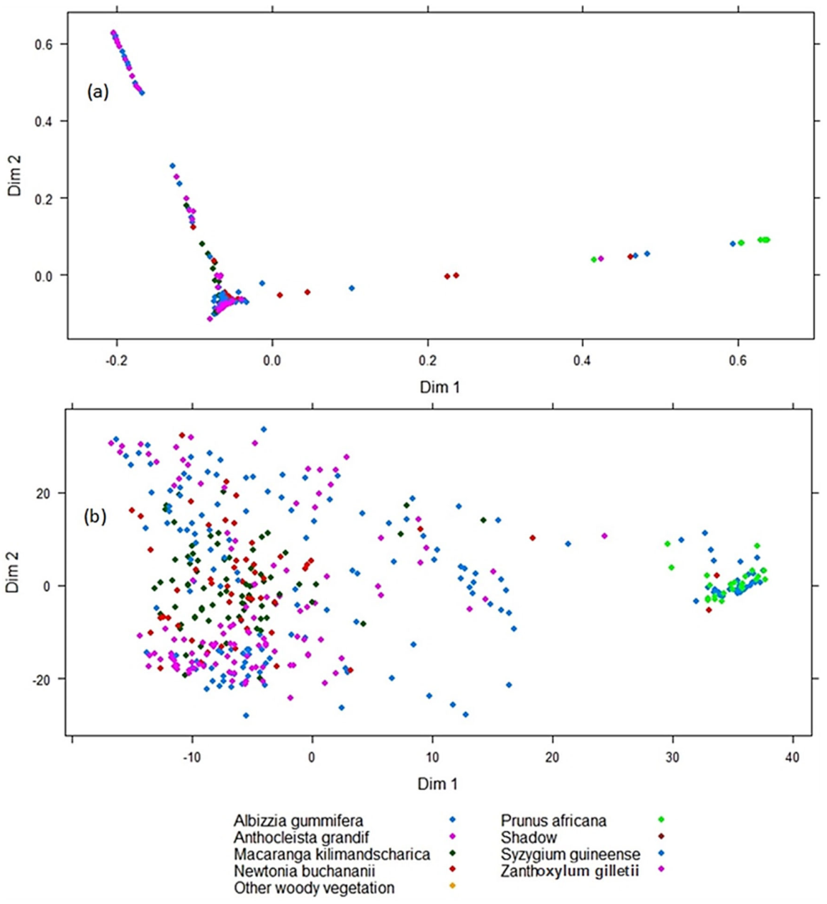
3.1. Spectral Separability between the Tree Species

The first step in mapping tree species is to figure out if the classes are spectrally different. Figure 3 shows the mean spectral signatures for the eight tree species in the study area. In the visible bands, Syzygium guineense has higher reflectance values compared to the other seven tree species which reflect almost the same. The Coastal band shows the highest reflectance values for all tree species. The difference in reflectance between Syzygium guineense and the other tree species keeps on increasing from the Coastal band towards the Red band.
The reflectance values in the Red Edge, Near Infrared 1, and Near Infrared 2 bands are generally higher for the deciduous and semi-deciduous tree species than for the evergreen tree species. Zanthoxylum gilletii and Albizzia gummifera showed the highest reflectance values and differ significantly from the others. Among the evergreen tree species, Prunus africana shows the highest reflectance values, followed by Anthocleista grandiflora. Syzygium guineense has notably low reflectance values. Among the three bands, Near Infrared 1 shows the highest reflectance values by all tree species. The Near Infrared 1 and Near Infrared 2 bands show the largest differences in reflectance between the seven tree species in the study area.
Figure 4 shows significant spectral overlaps between tree species. Band-specific within-species variance is evident, e.g., Syzygium guineense within-species variance is bigger in Coastal and Blue bands, and quite small in the Near Infrared 2. Zanthoxylum gilletii has the smallest within-species variance in the Red band, whereas the Coastal and Green bands show larger variances.
Table 2 is a matrix showing the inter-specific spectral separability of the tree species calculated from the WorldView-2 VNIR bands using the JM distance. The highest JM distances were reported for Syzygium guineense, i.e., values greater than 1. The lowest values were 0.42 for separability between Newtonia buchananii and Albizzia gummifera, and 0.43 for Newtonia buchananii and Anthocleista grandiflora. The highest values are shown in bold.

3.2. Optimization of Random Forest and Support Vector Machine

In all models, extracting the best performing ntree and mtry parameters to be used in training of the RF algorithm, repeated 10-fold cross-validation (CV) technique, dependent on the out-of-bag (OOB) error was applied. Using the same approach, the SVM parameters were optimized for the WorldView-2 dataset. The best parameters combinations under each of the four models are summarized in Table 3. As expected, the dataset produced by the combined oversampling and then downsampling techniques performed better than the others. For the R model, the default mtry value of 2 and ntree value of 3500 produced the lowest OOB error rate, 0.271 (Figure 5a). The SVM parameters, i.e., gamma and cost, were optimized for the WorldView-2 dataset, also using a 10-fold grid search approach. As seen in Figure 5b, a gamma value of 1 and a cost value of 100 yielded the best performance with a cross-validation error of 0.326. For the undersampled dataset, the best performance was an OOB error rate of 0.476 produced by mtry value of 2 and ntree value of 3500. The SVM yielded a gamma value of 0.01 and a cost value of 10, with a cross-validation error of 0.422.

3.3. Relative Importance of Variables

After running the classification models, the MDA provided the relative importance of each band (Figure 6). The most important spectral bands in all models, i.e., bands depicted by highest MDA were the Red, Red Edge, Near Infrared 1, and Near Infrared 2.
The classification models also evaluated the ability of the WorldView-2 spectral bands to detect the tree species. Figure 7 shows that the Red band was critical in the identification of especially Syzygium guineense, and also involved to a greater extent in mapping Albizzia gummifera, Anthocleista grandiflora, Prunus africana, and Zanthoxylum gilletii. The Near Infrared 1 band contributed significantly to the mapping of Albizzia gummifera and Prunus africana, as well as Anthocleista grandiflora, Macaranga kilimandscharica, Newtonia buchananii, and Zanthoxylum gilletii. The Red Edge band majorly contributed to the identification of Macaranga kilimandscharica and other woody vegetation, and, to a greater extent, shadow. The Near Infrared 2 band was helpful in the mapping of all tree species at different proportions, but it was very vital in the identification of Albizzia gummifera, Anthocleista grandiflora, and Prunus Africana.

3.4. Model Performance

Figure 8a shows RF multidimensional scaling (MDS) is a nice way to visualize (dis)similarity within and among tree species, using the proximity matrix calculated from the variables in the training dataset. SVM multidimensional scaling also visualizes (dis)similarity within and among tree species, using the test data, as seen in Figure 8b. The undersampled dataset performed poorly by attaining higher stress values, i.e., 2.41% for RF and 2.09% for SVM. The rest of the datasets performed fairly as their stress values were in the range of 1.41–1.89% for RF and SVM classifiers.
The confusion matrices in Table 4 are for RF and SVM classifiers, for the combined technique, and F1-scores were closest to their model mean. They were computed using the test data, which comprised 30% of the ground truth data.
The combined technique dataset achieved the highest average overall accuracy on both RF and SVM models, i.e., 73.2 ± 2.5% and 70.9 ± 2.7%, respectively. The average species F1-score was 68.56 ± 2.6% for RF and 64.64 ± 3.4% for SVM. The F1-score ranged between 18 and 100%. Syzygium guineense and Zanthoxylum gilletii are characterized with high accuracy and low variability, unlike Albizzia gummifera, Anthocleista grandiflora, and Newtonia buchananii, which had low variability across iterations and also low F1-score (Figure 9).
The undersampled data reported the lowest F1-score, i.e., 45.8 ± 5% for RF, compared to SVM’s 48 ± 6%, unlike the other datasets where RF performed better than SVM. The original dataset’s F1-score were 63.8 ± 3.9% for RF and 62.7 ± 4.3% for SVM. The oversampled dataset achieved F1-score values of 67.8 ± 4.1% and 63.6 ± 3.7% for RF and SVM, respectively (Figure 10).
The McNemar’s test, applied to test whether there was a significant difference between the two best maps produced by the RF and SVM models, using the combined oversampling and undersampling techniques, returned a Z value of 0.96 (Table 5). Thus, there were no significant differences (Z ≥ 1.96) at 95% confidence level, existing amongst the confusion matrices of the two classifiers.

3.5. The Spatial Distribution of the Endangered Tree Species

In showing the distribution of tree species in the study area, two classified maps, i.e., one by RF and the other by SVM, produced using the combined technique dataset, whose F1-score was closest to their model mean are used (Figure 11). These maps show that tree species distribution is not haphazard. In the northwestern part of the study area is the Macaranga kilimandscharica. Syzygium guineense is mostly occupying the lower and central parts of the study area. Zanthoxylum gilletii covers the central-eastern and western parts. A combination of other vegetation types can be seen dominating mostly the lower parts of the study area. The other tree species, i.e., Albizzia gummifera, Anthocleista grandiflora, Prunus africana, and Newtonia buchananii are found throughout the study area.
The RF and SVM classifiers show differences in the size of each class. Macaranga kilimandscharica shows an area of 45.2 ha and 44.1 ha for RF and SVM classifier, respectively (Table 6). Zanthoxylum gilletii reported 7.1 ha for RF and 7.2 ha for SVM, a negligible difference of 0.1% between them. For Syzygium guineense, there was a 0.8% difference between the two classifiers: RF recorded 9.6 ha and SVM recorded 10.6 ha. Newtonia buchananii reported a difference of 0.4 ha between the two classifiers. Anthocleista grandiflora had the second largest difference between the two classifiers, 1.8 ha, i.e., 13.4 ha for RF and 15.2 ha for SVM. Other woody vegetation showed a difference of 1.9 ha between RF and SVM classifiers. Shadow recorded 10.6 ha and 11.1 ha for RF classifier and SVM classifier, respectively. The areal coverage of Prunus Africana and Albizzia gummifera was insignificant compared to that of the other classes.

4. Discussion

4.1. Spectral Separability between the Tree Species

This study aimed to evaluate the impact of imbalanced data in mapping endangered trees species in a selectively logged sub-montane heterogeneous tropical forest using random forest and support vector machine classifiers, and WorldView-2 multispectral imagery. As seen in Figure 4, there are spectral overlaps within the tree species classes. The overlaps could be due to, among other reasons, the study area’s complex forest structure, because some stands were multi-storied and also some tree crowns were relatively small, thus the presence of mixed pixels [5]. This led to some of the misclassifications between species, which was in agreement with their inter-specific separability (Table 2). Newtonia buchananii, Anthocleista grandiflora, and Albizzia gummifera are examples of tree species with significantly low F1-scores. The J–M distance values showed that the species were not as separable as Syzygium guineense, Zanthoxylum gilletii, and Macaranga kilimandscharica, which indicated higher spectral separability values and were more separable, and therefore had higher F1-score values. In addition, very steep mountainous terrain and dense forest made it difficult to collect data in the field. This may have interfered with the quality of ground data used in the validation process. This research observed that higher spectral similarity within a class and higher spectral variability among classes led to higher classification accuracy. However, the contribution of the within- and among-species spectral variability on the classification accuracy of tropical tree species is poorly understood [17].

4.2. Relative Importance of Variables

In the classification process, the study was able to single out the most valuable bands, by making use of the variable importance (VI) measurement in the RF algorithm. RF uses the mean decrease in accuracy (MDA) and mean decrease in Gini (MDG) to evaluate the explanatory power of the input variables [37]. Generally, the best four bands in the classification process were the Red, Red Edge, Near Infrared 1, and Near Infrared 2 bands. This shows that both the visible and the infrared portions of the electromagnetic spectrum are quite relevant in the mapping of endangered tree species in the study area. The MDA was also used to show bands that were crucial in detecting particular tree species (Figure 7). However, both MDA and MDG are biased in adapting to the variables in the tree structure, hence larger values are provided than the actual value. Strobl et al. [45] point out that two indicators are unable to determine the explanatory power of variables in the classification process because they cannot distinguish false correlations due to data characteristics. Strobl et al. [45] developed a technique to evaluate the influence of conditional variable classification to solve this problem, but the technique is inconsistent in grasping the explanatory power variables [46]. Hur et al. [46] developed another technique based on the Shapley Value method on random forest regression. The determination of the relative importance of variables remains an active area of research.

4.3. Class Imbalance

The effect of unequal training class sizes for species classification from WorldView-2 imagery was reported in Section 3.4. The original dataset was imbalanced despite efforts to add samples of rare species, such as Prunus Africana and Albizzia gummifera, whose density has diminished in MKFR. The variation in the sample size across classes in the original dataset increased the rate of classification errors [26]. As expected, tree species with larger sample sizes had positive prediction bias, i.e., commission errors were greater than omission errors, and vice versa [18,40]. In addition,, species with small samples recorded high F1-score variability across iterations (Figure 9). The degree of bias in the model was minimized when the training data size was standardized across classes. The model that used the original dataset reported a reduced overall accuracy. In recent times, research shows that balanced data offers better overall classification performance [26,40]. The F1-score for the combined technique model was 68.56 ± 2.6% and 64.64 ± 3.4% for RF and SVM, respectively, whereas the unbalanced, original dataset reported F1-scores of 63.8 ± 3.9% for RF and 62.7 ± 4.3% for SVM. Previous studies have shown that the k-NN (k-nearest neighbor), RF, and SVM algorithms are affected by imbalanced training data [26]. Although these results are consistent with other studies using similar classification algorithms, they may not be directly comparable because of factors such as differences in the topography of the study area, size of samples, species diversity in the study area, a continuous closed canopy, size of the study area, and spectral and spatial resolutions of the images used.
The undersampling techniques reduce observation numbers from the majority class to make the dataset balanced. This technique may lead to the loss of important information in the training data. According to Graves et al. [18], lowering the number of the sampled common tree species while maintaining the species’ full range spectral variability solves the reduced overall accuracy problem. Spectral variability in data can be retained when using SVM algorithms by selecting data points on the border between classes to delineate the separation between them [44], or to iteratively prune the support vectors to attain the best separation between classes [47]. Another way is the manipulation of the SVM algorithm by adjusting margin variable misclassification costs, e.g., the cost of misclassifying a feature in the minority class is set higher than that of misclassifying a feature in the majority class [26]. However, the effects of these selection processes on bias in models and successive application to larger areas with many classes have not been quantified [18].
Apart from the techniques applied in this study to reduce class imbalance, other methods, e.g., balanced class weight, and generating synthetic data of the minority class that are similar to the original minority examples in the feature space using methods such as the synthetic minority over-sampling (SMOTE) technique [40], among others, can be used. In this study, the idea was to combine the undersampling and oversampling techniques to create a robust balanced dataset fit for model training.
According to Krawczyk [48], the imbalanced classification problem is not solved; at a time when we have such terms as big data, large neural network models, deep learning, and models such as the xgboost, solutions should be identified and addressed specifically for each training dataset [48].

4.4. Model Performance

In using an imbalanced dataset, the final classification under-predicts the classes with fewer samples, thus minority classes will have less effect on the accuracy compared to larger classes [49]. Therefore, test samples belonging to smaller classes are more often misclassified than those belonging to the dominant classes [26,40]. In such a case, a model may report a high accuracy level, but the map would not be useful. Accuracy is appropriate for balanced datasets but not good for imbalanced ones [18]. In some cases, the accuracy of samples in the smaller classes can be of greater importance than the contrary case [26,40]. This is the case in this research because the mapping of sparse tree species, e.g., Prunus Africana and Albizzia gummifera is crucial.
The balancing of the original dataset slightly improved the F1-scores for RF and SVM classifiers. Omission errors were recorded for each species, but Newtonia buchananii had the highest omission errors in all models. Newtonia buchananii and Anthocleista grandiflora exhibited a higher level of spectral confusion. This further degraded the F1-scores in all models, because tree species with low separability tend to have high misclassification rates. Furthermore, these tree species exhibited different crown color and density [50]. In addition,, because random sampling was used to collect field data, tree crowns used to train and validate the classifications of tree species are not distributed equally over the forest. The dense forest and rough mountainous terrain limited the places we could access within the forest. This may as well have influenced the outcome of the classification.
Finally, although error matrices are very crucial in comparing classification results, they only give an estimate of the accuracy of the classification, determined by the samples collected from the field. Thus, only biased conclusions can be made from such data [44]. Other metrics of model performance should be tried, e.g., balanced accuracy, bias score, or the F-score, among others [16].

4.5. The Spatial Distribution of Endangered Tree Species

This study found that, Macaranga kilimandscharica, an invasive species, mostly occupies the northwestern part of the study area. This tree species is found in areas that have experienced heavy intensive logging and forest disturbance. Logging activities have taken place in this area in the recent past. The RF and SVM classified maps of the study area have shown that Newtonia buchananii is more dominant than Syzygium guineense, Zanthoxylum gilletii, Anthocleista grandiflora, Albizzia gummifera, and Prunus africana. Both Prunus africana and Albizzia gummifera are hard to find in the study area. The same applies to Ocotea usambarensis. Once dominant in the wet forests of Mount Kenya, the endangered tree species are now rare.
In cases where differences in accuracy are marginal, i.e., a few percentage points apart, Janssen and van der Wel [51] propose that a statistically rigorous way must be used to compare the accuracies, and the results should be expressed with confidence limits. In this study, the McNemar test was used to evaluate the RF and SVM classification outputs of the combined technique dataset. The McNemar test was meant to indicate whether a difference of 3.9% was statistically important. A difference in accuracy between the confusion matrices of different WorldView-2 spectral subsets is statistically significant (p ≤ 0.05) if the Z value is more than 1.96 [44] The Z value was 0.96, meaning there is no significant difference between the two maps. Therefore, either of the two maps can be considered for conservation purposes.

5. Conclusions

This study aimed to assess the effects of imbalanced data on identifying and mapping trees species under threat in a selectively logged sub-montane heterogeneous tropical forest using RF and SVM classifiers and WorldView-2 multispectral imagery. The study obtained average F1-scores of 68.56 ± 2.6% and 64.64 ± 3.4% for RF and SVM, respectively, for the best model, the combined oversampling and undersampling technique. This was an improvement from the original imbalanced dataset. The F1-scores reported were directly related to the differences between the spectral variability within and among species. The most important spectral bands identified to have played a major role in mapping the endangered tree species in the study area were the Red, Red Edge, Near Infrared 1, and Near Infrared 2 bands. The tree species portrayed significant spectral overlaps, and this may have led to misclassification errors between classes. As well, difficult mountainous terrain and dense forest made it hard to collect data in the field, and this may have interfered with the quality of data, and thus contributed to increased classification errors.
Given the results presented here, the approach used in this study may serve as the basis for forest recovery initiatives in MKFR, an ecosystem that is considered a biodiversity hot-spot for conservation priorities. However, these applications are based on models of species classification that are not perfect [18]; therefore, more methods need to be developed to overcome the challenges caused by imbalanced data. Further research will target a larger study area and a higher number of tree species using VHR satellite data and object-based image analysis techniques.

Author Contributions

C.M.J.: conceptualization and methodology, C.M.J. & E.A.: data curation, E.A.: supervision, C.M.J.: validation, C.M.J. & E.A.: writing—review and editing. All authors have read and agreed to the published version of the manuscript.

Funding

This research did not receive any specific grant from funding agencies in the public, commercial, or not-for-profit sectors.

Data Availability Statement

Not applicable.

Conflicts of Interest

The authors have declared that no competing interests exist.

References

  1. Solberg, R.; Malnes, E.; Amlien, J.; Danks, F.; Haarpaintner, J.; Høgda, K.-A.; Johansen, B.E.; Karlsen, S.R.; Koren, H. State of the art for tropical forest monitoring by remote sensing. In A Review Carried out for the Ministry for the Environment of Norway and the Norwegian Space Centre; Norwegian Computing Centre: Oslo, Norway, 2008; pp. 1–76. [Google Scholar]
  2. Slik, J.W.F.; Arroyo-Rodrguez, V.; Aiba, S.-I.; Alvarez-Loayza, P.; Alves, L.F.; Ashton, P.; Balvanera, P.; Bastian, M.L.; Bellingham, P.J.; van den Berg, E.; et al. An estimate of the number of tropical tree species. Proc. Natl. Acad. Sci. USA 2015, 112, 7472–7477. [Google Scholar] [CrossRef] [PubMed] [Green Version]
  3. Wagner, F.H.; Ferreira, M.P.; Sanchez, A.; Hirye, M.C.M.; Zortea, M.; Gloor, E.; Phillips, O.L.; Filho, C.R.S.; Shimabukuro, Y.E.; Aragão, L.E.O.C. Individual tree crown delineation in a highly diverse tropical forest using very high-resolution satellite images. ISPRS J. Photogramm. Remote Sens. 2018, 145 Pt B, 362–377. [Google Scholar] [CrossRef]
  4. Ferreira, M.P.; Wagner, F.H.; Aragão, L.E.O.C.; Shimabukuro, Y.E.; de Souza Filho, C.R.S. Tree species classification in tropical forests using visible to shortwave infrared WorldView-3 images and texture analysis. ISPRS J. Photogramm. Remote Sens. 2019, 149, 119–131. [Google Scholar] [CrossRef]
  5. Immitzer, M.; Atzberger, C.; Koukal, T. Tree species classification with random forest using very high spatial resolution 8-band WorldView-2 satellite data. Remote Sens. 2012, 4, 2661–2693. [Google Scholar] [CrossRef] [Green Version]
  6. Nagendra, H.; Rocchini, D. High resolution satellite imagery for tropical biodiversity studies: The devil is in the detail. Biodiv. Conserv. 2008, 17, 3431–3442. [Google Scholar] [CrossRef]
  7. Clark, M.L.; Roberts, D.A.; Clark, D.B. Hyperspectral discrimination of tropical rain forest tree species at leaf to crown scales. Remote Sens. Environ. 2005, 96, 375–398. [Google Scholar] [CrossRef]
  8. Zhang, J.; Rivard, B.; Sánchez-Azofeifa, A.; Castro-Esau, K. Intra- and inter-class spectral variability of tropical tree species at La Selva, Costa Rica: Implications for species identification using HYDICE imagery. Remote Sens. Environ. 2006, 105, 129–141. [Google Scholar] [CrossRef]
  9. Trichon, V.; Julien, M.-P. Tree species identification on large-scale aerial photographs in a tropical rain forest, French Guiana-application for management and conservation. For. Ecol. Manag. 2006, 225, 51–61. [Google Scholar] [CrossRef] [Green Version]
  10. Somers, B.; Asner, G.P. Hyperspectral time series analysis of native and invasive species in Hawaiian rainforests. Remote Sens. 2012, 4, 2510–2529. [Google Scholar] [CrossRef] [Green Version]
  11. Féret, J.-B.; Asner, G.P. Semi-supervised methods to identify individual crowns of lowland tropical canopy species using imaging spectroscopy and LiDAR. Remote Sens. 2012, 4, 2457–2476. [Google Scholar] [CrossRef] [Green Version]
  12. Clark, M.L.; Roberts, D.A.; Clark, D.B. Species-Level Differences in Hyperspectral Metrics among Tropical Rainforest Trees as Determined by a Tree-Based Classifier. Remote Sens. 2012, 4, 1820–1855. [Google Scholar] [CrossRef] [Green Version]
  13. Papeş, M.; Tupayachi, R.; Martínez, P.; Peterson, A.T.; Asner, G.P.; Powell, G.V.N. Seasonal variation in spectral signatures of five genera of rainforest trees. IEEE J. Sel. Top. Appl. Earth Obs. Remote Sens. 2013; 6, 339–350. [Google Scholar] [CrossRef]
  14. Feret, J.B.; Asner, G.P. Tree species discrimination in tropical forests using airborne imaging spectroscopy. IEEE Trans. Geosci. Remote Sens. 2013, 51, 73–84. [Google Scholar] [CrossRef]
  15. Singh, M.; Evans, D.; Tan, B.S.; Nin, C.S. Mapping and Characterizing Selected Canopy Tree Species at the Angkor World Heritage Site in Cambodia Using Aerial Data. PLoS ONE 2015, 10, e0121558. [Google Scholar] [CrossRef]
  16. Baldeck, C.A.; Asner, G.P.; Martin, R.E.; Anderson, C.B.; Knapp, D.E.; Kellner, J.R.; Wright, S.J. Operational tree species mapping in a diverse tropical forest with airborne imaging spectroscopy. PLoS ONE 2015, 10, e0118403. [Google Scholar] [CrossRef]
  17. Ferreira, M.P.; Zortea, M.; Zanotta, D.C.; Shimabukuro, Y.E.; de Souza Filho, C.R. Mapping tree species in tropical seasonal semi-deciduous forests with hyperspectral and multispectral data. Remote Sens. Environ. 2016, 179, 66–78. [Google Scholar] [CrossRef]
  18. Graves, S.J.; Asner, G.P.; Martin, R.E.; Anderson, C.B.; Colgan, M.S.; Kalantari, L.; Bohlman, S.A. Tree species abundance predictions in a tropical agricultural landscape with a supervised classification model and imbalanced data. Remote Sens. 2016, 8, 161. [Google Scholar] [CrossRef] [Green Version]
  19. Mutanga, O.; Adam, E.; Cho, M.A. High density biomass estimation for wetland vegetation using WorldView-2 imagery and random forest regression algorithm. Int. J. Appl. Earth Obs. Geoinf. 2012, 18, 399–406. [Google Scholar] [CrossRef]
  20. NEMA (National Environment Management Authority). Kenya State of the Environment and Outlook 2010; Supporting the Delivery of Vision 2030. Available online: http://www.enviropulse.org/documents/Kenya_SOE.pdf (accessed on 3 January 2019).
  21. KWS (Kenya Wildlife Service). Mt Kenya Ecosystem Management Plan 2010–2020. Available online: http://www.kws.go.ke/file/1470/download?token=1lO6G3zI (accessed on 16 February 2019).
  22. Wass, P. Kenya’s Indigenous Forests: Status, Management and Conservation; IUCN: Gland, Switzerland; Cambridge, UK, 1995; 205p. [Google Scholar]
  23. Bussmann, R.W. Destruction and management of Mount Kenya’s forests. Ambio 1996, 25, 314–317. [Google Scholar]
  24. Ng’eno, J.K. Kenya. Proceedings of Country report to the FAO International Technical Conference on Plant Genetic Resources, Leipzig, Germany, 17–23 June 1996. [Google Scholar]
  25. KFS (Kenya Forest Service). Mt. Kenya Forest Reserve Management Plan 2010–2019. Available online: http://www.kenyaforestservice.org/documents/MtKenya.pdf (accessed on 3 January 2019).
  26. Maxwell, A.E.; Warner, T.A.; Fang, F. Implementation of machine-learning classification in remote sensing: An applied review. Int. J. Remote Sens. 2018, 39, 2784–2817. [Google Scholar] [CrossRef] [Green Version]
  27. Bussmann, R.W. Stand structure and regeneration of the subalpine Hagenia abyssinica forest of Mt. Kenya. Bot. Act. 1997, 110, 473–480. [Google Scholar] [CrossRef]
  28. Baker, B.H. Geology of the Mount Kenya Area. Geol. Surv. Kenya Rep. 1967, 79, 464–465. [Google Scholar]
  29. Nyongesa, K.W.; Vacik, H. Evaluating management strategies for Mount Kenya Forest Reserve and National Park to reduce fire danger and address interests of various stakeholders. Forests 2019, 10, 426. [Google Scholar] [CrossRef] [Green Version]
  30. Ogondo, J.A. Geomorphological formation of Mount Kenya. Proceedings of Kenya National Commission for UNESCO, Stakeholders sensitization Workshop on the extension of Mt. Kenya World Heritage Site, at Sportsman’s Arm Hotel, Nanyuki, Kenya, 27–28 August 2009. [Google Scholar] [CrossRef]
  31. DigitalGlobe. The Benefits of the 8 Spectral Bands of WorldView-2. Available online: https://dg-cms-uploads-production.s3.amazonaws.com/uploads/document/file/35/DG-8SPECTRAL-WP_0.pdf (accessed on 2 February 2019).
  32. Jensen, J.R. Introductory Digital Image Processing: A Remote Sensing Perspective, 3rd ed.; Prentice Hall: Upper Saddle River, NJ, USA, 2005; pp. 210–215. [Google Scholar]
  33. GoK (Government of Kenya). Fifth National Report to the Conference of Parties to the Convention on Biological Diversity. Available online: https://www.cbd.int/doc/world/ke/ke-nr-05-en.pdf (accessed on 16 June 2019).
  34. GoK (Government of Kenya). The Wildlife Conservation and Management Act, 2013; No. 47 of 2013; GoK: Nairobi, Kenya, 2013. [Google Scholar]
  35. Richards, J.A.; Jia, X. Remote Sensing Digital Image Analysis: An Introduction, 3rd ed.; Springer-Verlag: Berlin/Heidelberg, Germany, 1999. [Google Scholar]
  36. Kailath, T. The divergence and bhattacharyya distance measures in signal selection. IEEE Trans. Commun. Technol. 1967, 15, 52–60. [Google Scholar] [CrossRef]
  37. Breiman, L. Random forests. Machin. Learn. 2001, 45, 5–32. [Google Scholar] [CrossRef] [Green Version]
  38. Vapnik, V. The Nature of Statistical Learning Theory, 2nd ed.; Springer-Verlag: New York, NY, USA, 2000. [Google Scholar]
  39. Kuter, S. Completing the machine learning saga in fractional snow cover estimation from MODIS Terra reflectance data: Random forests versus support vector regression. Remote Sens. Environ. 2021, 255, 112294. [Google Scholar] [CrossRef]
  40. Chawla, N.V.; Japkowicz, N.; Kolcz, A. Editorial: Special issue on learning from imbalanced data sets. ACM SIGKDD Explor. Newsl. 2004, 6, 1–6. [Google Scholar] [CrossRef]
  41. Borg, I.; Groenen, P.J.F. Modern Multidimensional Scaling: Theory and Applications, 2nd ed.; Springer Science + Business Media: Berlin, Germany, 2005. [Google Scholar]
  42. NCSS. Chapter 435. Multidimensional Scaling. Available online: https://ncss-wpengine.netdna-ssl.com/wp-content/themes/ncss/pdf/Procedures/NCSS/Multidimensional_Scaling.pdf (accessed on 18 November 2021).
  43. Buja, A.; Swayne, D.F.; Littman, M.L.; Dean, N.; Hofmann, H.; Chen, L. Data Visualization with Multidimensional Scaling. J. Comput. Graph. Stat. 2007, 17, 444–472. [Google Scholar] [CrossRef]
  44. Foody, G.M.; Mathur, A. Toward intelligent training of supervised image classifications: Directing training data acquisition for SVM classification. Remote Sens. Environ. 2004, 93, 107–117. [Google Scholar] [CrossRef]
  45. Strobl, C.; Boulesteix, A.-L.; Kneib, T.; Augustin, T.; Zeileis, A. Conditional variable importance for random forests. BMC Bioinform. 2008, 9, 307. [Google Scholar] [CrossRef] [Green Version]
  46. Hur, J.-H.; Ihm, S.-Y.; Park, Y.-H. A variable impacts measurement in random forest for mobile cloud computing. Wirel. Commun. Mob. Comput. 2017, 2017, 1–13. [Google Scholar] [CrossRef] [Green Version]
  47. Chen, X.; Gerlach, B.; Casasent, D. Pruning support vectors for imbalanced data classification. Proceedings of International Joint Conference on Neural Networks, Montreal, QC, Canada, 31 July–4 August 2005; pp. 1883–1888. [Google Scholar] [CrossRef]
  48. Krawczyk, B. Learning from imbalanced data: Open challenges and future directions. Prog. Artif. Intell. 2016, 5, 221–232. [Google Scholar] [CrossRef] [Green Version]
  49. He, H.; Garcia, E.A. Learning Form Imbalanced Data. IEEE Trans. Knowl. Data Eng. 2009, 21, 1263–1284. [Google Scholar] [CrossRef]
  50. Adam, E.; Mutanga, O.; Odindi, J.; Abdel-Rahman, E.M. Land-use/cover classification in a heterogeneous coastal landscape using RapidEye imagery: Evaluating the performance of random forest and support vector machines classifiers. Int. J. Remote Sens. 2014, 35, 3440–3458. [Google Scholar] [CrossRef]
  51. Janssen, L.L.F.; van der Wel, F.J.M. Accuracy assessment of satellite-derived land-cover data—A review. Photogramm. Eng. Remote Sens. 1994, 60, 419–426. [Google Scholar]
Figure 1. WorldView-2 false-color composite (near-infrared 2: yellow: coastal) of the study area showing tree crowns identified to the species level and other forest landscape features in the field.
Remotesensing 13 04970 g001
Figure 2. Samples of endangered tree species in the study area.
Remotesensing 13 04970 g002
Figure 3. Tree species mean spectral signatures derived from the WorldView-2 data.
Remotesensing 13 04970 g003
Figure 4. Box-whisker plots showing tree species mean reflectance values derived from WorldView-2 data. The central lines within each box represent the medians, while the top and bottom edges of the boxes are the upper and lower quartiles, respectively. The dots represent the outlier values within tree species. Full species names for each species code are given in Table 1.
Remotesensing 13 04970 g004
Figure 5. Optimization by 10—fold cross—validation: (a) random forest parameters (mtry and ntree), and (b) support vector machine parameters (gamma and cost).
Remotesensing 13 04970 g005
Figure 6. The relative importance of WorldView-2 bands in discriminating between different tree species as measured by RF classifier.
Remotesensing 13 04970 g006
Figure 7. The mean decrease accuracy (MDA) values show the relationship between each tree species and WorldView-2 spectral bands as measured by the RF classifier. Full species names for each species code are given in Table 1.
Remotesensing 13 04970 g007
Figure 8. Visualizing tree species (dis)similarity using MDS scaling: (a) RF; (b) SVM.
Remotesensing 13 04970 g008
Figure 9. Species-level F1-score for the combined oversampling and undersampling technique: (a) RF; (b) SVM.
Remotesensing 13 04970 g009
Figure 10. Model-level F1-score for the datasets: (a) RF; (b) SVM.
Remotesensing 13 04970 g010
Figure 11. Classification maps of tree species in Mt. Kenya Forest, obtained using (a) random forest and (b) support vector machine.
Remotesensing 13 04970 g011
Table 1. List of tree species, codes, family, leafy phenology, diameter at breast height (DBH), number of individual tree crowns, and composition of training and test data for each species used to map trees in Mt. Kenya Forest Reserve.
Botanical NameCodeFamilyLeaf PhenologyDBH (m)Train DataTest DataTotal
Macaranga k.MKEuphorbiaceaeSemi-deciduous0.30–0.57562480
Zanthoxylum g.ZGRutaceaeSemi-deciduous0.97–3.00562480
Syzygium g.SGMyrtaceaeEvergreen1.00–2.50562480
Newtonia b.NBFabaceaeDeciduous1.50–4.50562480
Anthocleista g.AnGGentianaceaeEvergreen1.01–2.50361551
Prunus a.PARosaceaeEvergreen1.24–3.50221032
Albizzia g.AlGFabaceaeDeciduous 1.37–4.0020828
Other woody vegetationOWV---------562480
ShadowSD---------562480
Table 2. Tree species’ inter-specific spectral separability as calculated by the Jeffries–Matusita distance (Equation (1)). The bold shows those species which are separable and those not separable (not in bold).
SGZGAnGAlGPANBMK
SG 1.371.211.231.271.251.16
ZG 1.010.751.050.891.22
AnG 0.510.590.430.66
AlG 0.650.420.87
PA 0.580.90
NB 0.74
MK
Table 3. The RF and SVM model optimization parameters.
ModelTrain
Data per Species
RFSVM
mtry ntreeOOB ErrorGammaCostCV Error
Original datasetRefer to Table 1315000.3770.0110000.387
Oversampling technique56445000.2790.0110000.327
Undersampling technique20235000.4760.01100.422
Combined techniquevaried235000.27111000.326
The sampling techniques were only applied to training data to avoid model overfitting.
Table 4. Confusion matrices for (a) RF algorithm and (b) SVM algorithm, for the combined oversampling and undersampling technique. Full species names for each species code are given in Table 1.
(a) Random Forest
AlGAnGMKNBOWVPASDSGZGTotalUA (%)
AlG4113001001040.0
AnG0941220001850.0
MK00162020002080.0
NB3429100012045.0
OWV00021700012085.0
PA0015160001346.2
SD000000230023100.0
SG000000023023100.0
ZG11023001223073.3
Total81524242410242424177
PA (%)50.060.066.737.570.860.090.090.080.0
Overall accuracy = 72.9% F1-score = 68.0%
(b) Support Vector Machine algorithm
AlGAnGMKNBOWVPASDSGZGTotalUA (%)
AlG311210000837.5
AnG1832221012040.0
MK00153021002171.4
NB3427100011838.9
OWV00021700001989.5
PA1126260001833.3
SD000000220022100.0
SG000000024024100.0
ZG01121000222781.5
Total81524242410242424177
PA (%)37.553.362.529.270.860.080.0100.070.8
Overall accuracy = 70.1% F1-score = 64.2%
Table 5. McNemar’s test results to compare RF and SVM classification models using the combined oversampling and undersampling technique.
ClassifierRF
SVM CCICTotal
CC9811111
IC165266
Total11463177
CC stands for correctly classified and IC is for incorrectly classified samples.
Table 6. Area coverage in hectares and percentage of the classes using RF and SVM classifiers.
ClassesRF Classified Area (ha)Percentage (%)SVM Classified Area (ha)Percentage (%)
Macaranga kilimandscharica45.234.844.133.9
Zanthoxylum gilletii7.15.57.25.6
Syzygium guineense9.67.410.68.2
Newtonia buchananii23.618.123.217.8
Anthocleista grandiflora13.410.315.211.7
Prunus africana0.00.00.00.0
Albizzia gummifera0.00.00.00.0
Other woody vegetation20.515.818.614.3
Shadow10.68.111.18.5
Total130100130100
Publisher’s Note: MDPI stays neutral with regard to jurisdictional claims in published maps and institutional affiliations.

